Homework 4 Solutions
ChE 621 — Thermodynamics.
Problem 1
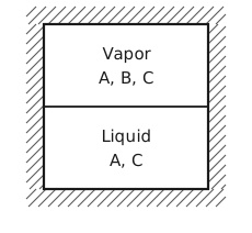
Figure 1 The insulated bomb. A square vessel with hatched walls all round, for the insulation. A horizontal line across the middle is the liquid surface. The upper half is labelled Vapor, with the species A, B, C, and the lower half Liquid, with the species A, C.
The reaction \(\mathrm{A} \rightleftharpoons 2\,\mathrm{B} + \mathrm{C}\) occurs in the gas phase only, and B is in the vapor phase only.
At equilibrium
but
Now that all variations are independent, we must have at equilibrium that
Problem 2
Part (a): \(n\) components in \(π\) phases at fixed \(T\), \(P\) and moles
In this case the necessary condition for equilibrium at fixed \(T\) and \(P\) is
The closed system constraints are
This gives us
The displacements are now independent so that we find
for all \(i\).
Part (b): two subsystems behind a rigid membrane permeable only to A
The necessary condition for equilibrium is:
Fixed temperature and the rigid membrane lead to the following constraints:
The total volume \(V_{1} + V_{2}\) is then fixed as well. Since the membrane is only permeable to A, the following constraints are valid:
Based on the closed system constraints
we have
Substituting these constraints into the equilibrium equation, we have
The displacement \(\mathrm{d}N_{\mathrm{A}1}\) is now independent, so its coefficient must be zero. This leads to
Because the membrane is rigid, the two subsystems cannot exchange volume, so the pressures \(P_{1}\) and \(P_{2}\) need not be equal. Because B and C cannot cross the membrane, their chemical potentials need not be equal on the two sides either.
Problem 3
The equilibrium constant as a function of temperature
For \(\mathrm{N}_{2} + 3\,\mathrm{H}_{2} \rightarrow 2\,\mathrm{NH}_{3}\) the stoichiometric coefficients are \(ν_{\mathrm{N}_{2}} = -1\), \(ν_{\mathrm{H}_{2}} = -3\) and \(ν_{\mathrm{NH}_{3}} = 2\). The tabulated formation values are for 1 mol of \(\mathrm{NH}_{3}\), so for the reaction as written, at \(T_{0} = 298.15\) K,
The heat capacity of reaction, \(Δ\tilde{C}_{p} = ΔA + ΔB\,T + ΔC\,T^{2} + ΔD/T^{2}\), with \(ΔX = \sum_{i} ν_{i} X_{i}\):
The enthalpy of ideal gases is a function of only temperature:
The Gibbs–Helmholtz equation, \(\mathrm{d}\left(Δ\tilde{G}^{θ}/T\right)/\mathrm{d}T = -Δ\tilde{H}^{θ}/T^{2}\), integrated from \(T_{0}\) gives
where the constant \(I = -115.18\) J/(mol K) is fixed by \(Δ\tilde{G}^{θ}(T_{0}) = -32.900\) kJ/mol. Then
\(T\) (K) |
\(Δ\tilde{H}^{θ}\) (kJ/mol) |
\(Δ\tilde{G}^{θ}\) (kJ/mol) |
\(K\) |
|---|---|---|---|
400 |
−96.43 |
−11.97 |
36.6 |
600 |
−103.21 |
31.80 |
\(1.70 \times 10^{-3}\) |
700 |
−105.98 |
54.53 |
\(8.53 \times 10^{-5}\) |
800 |
−108.37 |
77.62 |
\(8.55 \times 10^{-6}\) |
The extent of reaction against pressure
Starting from 1 mol \(\mathrm{N}_{2}\) and 3 mol \(\mathrm{H}_{2}\), at extent \(ξ\) the mixture holds
For an ideal-gas mixture, with the standard-state pressure \(P^{θ} = 1\) atm,
Taking the square root, and using \(ξ(2 - ξ) = 1 - (1 - ξ)^{2}\),
which is plotted in Figure 2 and tabulated in Table 2.
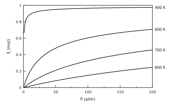
Figure 2 Extent of the ammonia synthesis against pressure. The extent of reaction \(ξ\), in mol, from 0 to 1, is plotted against the pressure \(P\) from 1 to 200 atm, for 1 mol \(\mathrm{N}_{2}\) and 3 mol \(\mathrm{H}_{2}\) fed. There are four curves, labelled at their right-hand ends. At 400 K the extent starts at 0.66 at 1 atm, climbs steeply and levels off near 0.97. At 600 K it rises from almost zero to 0.71 at 200 atm, at 700 K to 0.46 and at 800 K to 0.25, each curve rising more slowly and more nearly straight than the one above it.
\(P\) (atm) |
\(ξ\) at 400 K |
\(ξ\) at 600 K |
\(ξ\) at 700 K |
\(ξ\) at 800 K |
|---|---|---|---|---|
1 |
0.664 |
0.026 |
0.006 |
0.002 |
10 |
0.888 |
0.193 |
0.055 |
0.018 |
50 |
0.950 |
0.479 |
0.209 |
0.083 |
100 |
0.964 |
0.604 |
0.326 |
0.149 |
200 |
0.975 |
0.708 |
0.458 |
0.246 |
The reaction is exothermic, so \(K\) and the extent fall as the temperature rises. It also reduces the number of moles of gas from 4 to 2, so the extent rises with pressure. Equilibrium alone would favor low temperature, but the reaction is too slow there, which is why the Haber process runs at high pressure and moderate temperature over a catalyst.
Problem 4
Part (a): the Gibbs function along an isotherm
To produce isotherms of \(\tilde{G}(P, T) - \tilde{G}^{\ominus}(T)\) against \(P\):
Pick \(\tilde{V}\).
Calculate \(P\) from the equation of state.
Calculate \(\tilde{G}(P, T) - \tilde{G}^{\ominus}(T)\) from the above equation.
Repeat steps 1 to 3 to generate many pairs of \(\left[P, \tilde{G}(P, T) - \tilde{G}^{\ominus}(T)\right]\) data points.
Part (b): the Gibbs function isotherms and the vapor pressure of ethane
The saturation pressure is where the liquid and vapor branches cross: \(P^{*}_{\mathrm{RK}} = 14.1\) bar at \(T = 250\) K (Figure 3), \(P^{*}_{\mathrm{RK}} = 26.4\) bar at \(T = 275\) K (Figure 4) and \(P^{*}_{\mathrm{RK}} = 44.2\) bar at \(T = 300\) K (Figure 5).
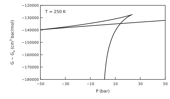
Figure 3 The Gibbs function of ethane at 250 K. \(G - G_{\mathrm{o}}\), in cm³ bar/mol, from −180000 to −120000, is plotted against \(P\) from −50 to 50 bar. A nearly straight, gently rising line runs across the whole plot: the liquid branch, which continues to negative pressures. A second branch rises steeply from the bottom of the plot near 0 bar and bends over: the vapor branch. It crosses the liquid line near 13 bar and ends in a sharp cusp near 24 bar and −127000, from which a short curved branch runs back down to the left and joins the liquid line at the left edge of the plot.
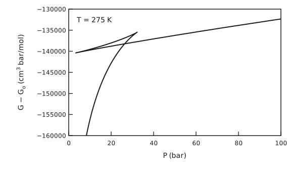
Figure 4 The Gibbs function of ethane at 275 K. \(G - G_{\mathrm{o}}\), in cm³ bar/mol, from −160000 to −130000, is plotted against \(P\) from 0 to 100 bar. The nearly straight liquid line rises gently from about 3 bar to the right edge. The vapor branch rises steeply from the bottom of the plot near 8 bar, crosses the liquid line near 26 bar and ends in a cusp near 32 bar, from which a short curved branch runs back down to meet the liquid line at its left end, near 3 bar.
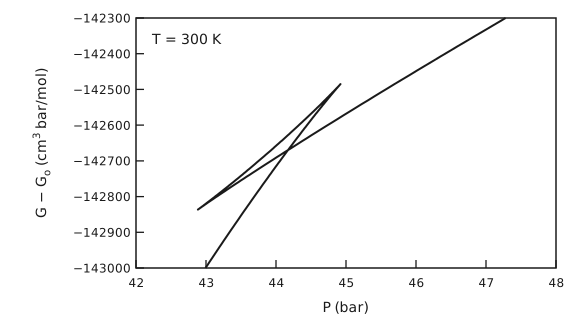
Figure 5 The Gibbs function of ethane at 300 K. \(G - G_{\mathrm{o}}\), in cm³ bar/mol, from −143000 to −142300, is plotted against \(P\) from 42 to 48 bar, a narrow window round the crossing. The vapor branch rises steeply from the bottom of the plot near 43 bar to a cusp near 44.9 bar. The liquid branch rises more gently from a cusp near 42.9 bar to the top right of the plot. The two cusps are joined by a short, nearly straight branch, which makes a thin triangle with the other two. The liquid and vapor branches cross near 44.2 bar.
At the critical temperature, 305.4 K, the loop has shrunk to a point: the liquid and vapor branches merge into one smooth curve with no crossing (Figure 6), so there is no vapor pressure. The bend of the curve is sharpest at the critical point, \(P_{\mathrm{c}} = 48.8\) bar, where \((\partial P / \partial \tilde{V})_{T} = 0\) and the curvature, \((\partial \tilde{V} / \partial P)_{T}\), grows without bound.
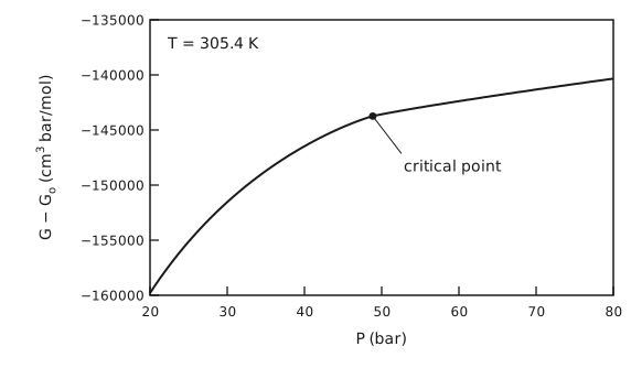
Figure 6 The Gibbs function of ethane at 305.4 K. \(G - G_{\mathrm{o}}\), in cm³ bar/mol, from −160000 to −135000, is plotted against \(P\) from 20 to 80 bar. The curve is a single smooth line that rises steeply at low pressure and more gently at high pressure, with no loop and no crossing. A dot marks the critical point, near 48.8 bar and −143700, where the bend is sharpest.
The experimental vapor pressures are 13, 25 and 43.2 atm, that is 13.2, 25.3 and 43.8 bar. Table 3 compares them with the predictions.
\(T\) (K) |
\(P^{*}_{\mathrm{RK}}\) (bar) |
\(P^{*}_{\exp}\) (bar) |
deviation |
|---|---|---|---|
250 |
14.1 |
13.2 |
+7.1 % |
275 |
26.4 |
25.3 |
+4.0 % |
300 |
44.2 |
43.8 |
+0.9 % |
The Redlich–Kwong equation overpredicts the vapor pressure at all three temperatures. The error is about 1 % at 300 K and grows to about 7 % at 250 K. Its constants \(a\) and \(b\) come from the critical point alone, so it is most accurate near \(T_{\mathrm{c}}\) and less so at lower reduced temperatures. Correcting this is what the acentric factor in later cubic equations, such as Soave–Redlich–Kwong, is for.
Part (c): the Helmholtz function along an isotherm
(Alternatively, \(\tilde{A} = \tilde{G} - P\tilde{V}\) will give the same result.) Figure 7 shows \(A\) against \(\tilde{V}\) at 305.4 and 300 K.
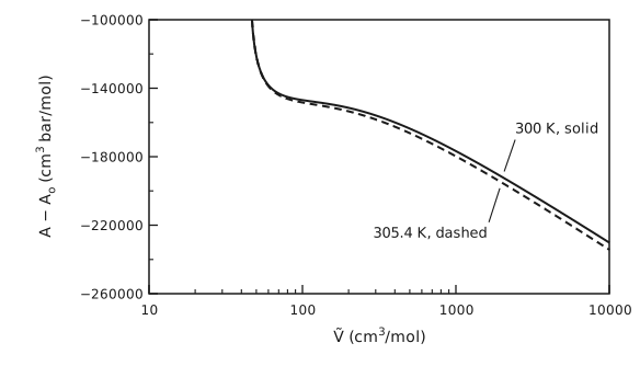
Figure 7 The Helmholtz function of ethane at 305.4 and 300 K. \(A - A_{\mathrm{o}}\), in cm³ bar/mol, from −260000 to −100000, is plotted against \(\tilde{V}\), in cm³/mol, on a logarithmic axis from 10 to 10000. Both curves fall steeply from the top of the plot just above 45 cm³/mol, flatten into a shoulder between about 80 and 300 cm³/mol, and then fall steadily to the right. The two curves almost coincide. The 300 K curve, solid and labelled, lies slightly above the 305.4 K curve, dashed and labelled, and the gap widens a little at large volumes.
Part (d): binodal and spinodal points at 300 K
Figure 8 shows the pressure against volume at 300 K, and Figure 9 and Figure 10 the Gibbs and Helmholtz functions with the same points marked.
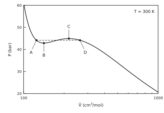
Figure 8 The 300 K isotherm of ethane. \(P\), in bar, from 20 to 60, is plotted against \(\tilde{V}\), in cm³/mol, on a logarithmic axis from 100 to 1000. The isotherm falls steeply from the top left, dips to a shallow minimum, rises to a shallow maximum and then falls steadily to the bottom right. A dashed horizontal tie line at about 44.2 bar runs from point A on the liquid side to point D on the vapor side. Point B is the minimum, just below the tie line, and point C the maximum, just above it.
Volumes less than A are stable. Volumes and pressures between A and B are metastable. Volumes and pressures between B and C are unstable. Volumes and pressures between C and D are metastable. Volumes greater than D are stable.
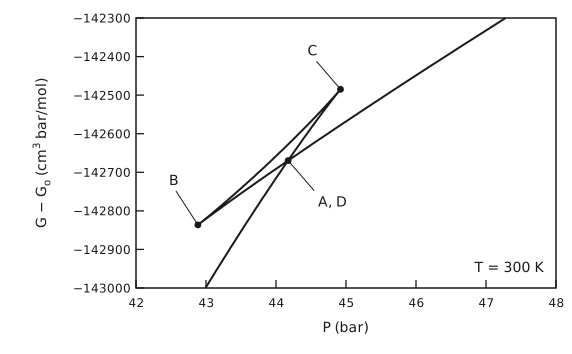
Figure 9 The 300 K Gibbs function with the points marked. The 300 K Gibbs function plot again: \(G - G_{\mathrm{o}}\) from −143000 to −142300 cm³ bar/mol against \(P\) from 42 to 48 bar. Point B is the cusp at the lower left, near 42.9 bar, and point C the cusp at the upper right, near 44.9 bar. Points A and D coincide at the crossing of the liquid and vapor branches, near 44.2 bar.
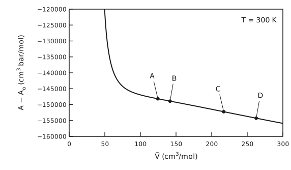
Figure 10 The 300 K Helmholtz function with the points marked. \(A - A_{\mathrm{o}}\), in cm³ bar/mol, from −160000 to −120000, is plotted against \(\tilde{V}\) from 0 to 300 cm³/mol on a linear axis. The curve falls steeply from the top of the plot just above 45 cm³/mol, bends sharply near 70 cm³/mol and then falls slowly and almost straight. Points A, B, C and D sit on this nearly straight part, at about 125, 142, 217 and 263 cm³/mol.
Note that the second derivative of \(A\) goes through zero and changes sign at B and C, that is, these are inflection points. They are difficult to make out because we are close to the critical point and \(A\) is very flat in between the binodal (and spinodal) points.
The liquid and vapor in equilibrium at 300 K are the binodal points A and D, at \(P^{*} = 44.2\) bar, with \(\tilde{V}^{\mathrm{L}} = 124.5\) cm³/mol and \(\tilde{V}^{\mathrm{V}} = 262.5\) cm³/mol. The spinodal points B and C lie at 141.5 and 217.0 cm³/mol. With the molar mass of ethane, \(M = 30.07\) g/mol, the densities are
Problem 5
Part (a): the normal boiling point
Part (b): the triple point
Part (c): the heat of evaporation at the normal boiling point
Assume the vapor phase behaves like an ideal gas:
Substituting \(T_{\mathrm{b}} = 2006.05\) K, we get \(Δ\tilde{H}^{\mathrm{lv}} = 216.45\) kJ/mol.
Part (d): the heat of melting at the triple point
but we don’t know \(Δ\tilde{V}^{\mathrm{sl}}\). At the triple point, all three phases are in equilibrium, and going from solid to vapor directly or by way of the liquid (Figure 11) we have
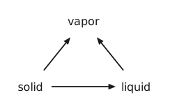
Figure 11 Solid to vapor, directly or through the liquid. Three words at the corners of a triangle: solid at the lower left, liquid at the lower right and vapor at the top. Arrows run from solid to liquid, from solid to vapor and from liquid to vapor.
Again assume an ideal-gas vapor phase:
Part (e): the difference between the heat capacities
Part (f): what else the phase diagram needs
We need to calculate the S-L boundary. According to Equation (1), we need both \(Δ\tilde{H}^{\mathrm{sl}}\) and \(Δ\tilde{V}^{\mathrm{sl}}\). \(Δ\tilde{H}^{\mathrm{sl}}\) is given in part (d), so what is still needed are the liquid and solid densities.
Problem 6
The enthalpy, entropy and Gibbs energy
With the reference state at 298 K and the entropy reference at 0 K, the enthalpy and the entropy of each form at 1 bar (constant pressure) are:
Reading the tabulated \(\tilde{H}_{\mathrm{f},298}\) in J/mol and \(\tilde{S}_{\mathrm{f},298}\) in J/(mol K), and with \(D = 0\) for both, these become, in J/mol and J/(mol K),
\(T\) (K) |
\(\tilde{H}_{α}\) (kJ/mol) |
\(\tilde{H}_{γ}\) (kJ/mol) |
\(\tilde{S}_{α}\) (kJ/(mol K)) |
\(\tilde{S}_{γ}\) (kJ/(mol K)) |
|---|---|---|---|---|
298 |
0.00 |
10.19 |
0.0273 |
0.0355 |
500 |
5.11 |
15.71 |
0.0404 |
0.0497 |
1000 |
21.35 |
30.87 |
0.0623 |
0.0705 |
1500 |
50.71 |
48.13 |
0.0856 |
0.0844 |
1800 |
78.79 |
59.51 |
0.1026 |
0.0913 |
\(T\) (K) |
\(\tilde{G}_{α}\) (kJ/mol) |
\(\tilde{G}_{γ}\) (kJ/mol) |
\(\tilde{G}_{γ} - \tilde{G}_{α}\) (kJ/mol) |
|---|---|---|---|
298 |
−8.14 |
−0.40 |
7.74 |
500 |
−15.09 |
−9.12 |
5.97 |
1000 |
−40.93 |
−39.63 |
1.30 |
1500 |
−77.69 |
−78.53 |
−0.84 |
1800 |
−105.85 |
−104.92 |
0.94 |
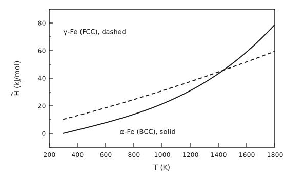
Figure 12 Enthalpy of \(α\)- and \(γ\)-iron. \(\tilde{H}\), in kJ/mol, from −10 to 90, is plotted against \(T\) from 298 to 1800 K. The \(α\)-Fe (BCC) curve, solid, starts at 0 at 298 K and curves upward ever more steeply to about 79 kJ/mol at 1800 K. The \(γ\)-Fe (FCC) curve, dashed, starts at 10.2 kJ/mol and rises almost linearly to about 60 kJ/mol. The two cross near 1430 K.
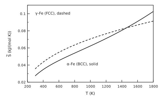
Figure 13 Entropy of \(α\)- and \(γ\)-iron. \(\tilde{S}\), in kJ/(mol K), from 0.02 to 0.11, is plotted against \(T\) from 298 to 1800 K. Both curves rise and bend over. The \(γ\)-Fe (FCC) curve, dashed, starts higher, at 0.036, and the \(α\)-Fe (BCC) curve, solid, starts at 0.027 but rises faster, crosses the dashed curve near 1460 K and ends higher, at 0.103 against 0.091.
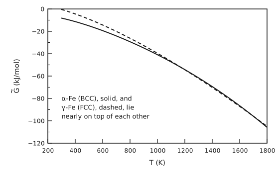
Figure 14 Gibbs energy of \(α\)- and \(γ\)-iron. \(\tilde{G}\), in kJ/mol, from −120 to 0, is plotted against \(T\) from 298 to 1800 K. Both curves fall and bend downward, from about −8 kJ/mol for \(α\)-Fe (BCC, solid) and −0.4 kJ/mol for \(γ\)-Fe (FCC, dashed) at 298 K to about −105 kJ/mol at 1800 K. Above about 1000 K the two lie nearly on top of each other.
What the Gibbs energies show
On the scale of Figure 14 the two Gibbs energies are almost indistinguishable at high temperature: they differ by less than 1 kJ/mol out of about 80. Plotting the difference, Figure 15, shows what is going on:
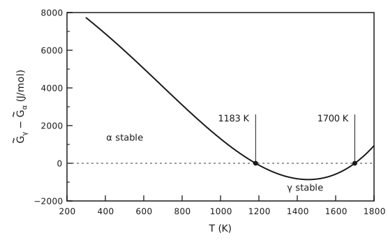
Figure 15 The Gibbs energy difference between \(γ\)- and \(α\)-iron. \(\tilde{G}_{γ} - \tilde{G}_{α}\), in J/mol, from −2000 to 8000, is plotted against \(T\) from 298 to 1800 K, with a dotted line at zero. The difference starts at about 7700 J/mol at 298 K, falls through zero at 1183 K, reaches a minimum of about −860 J/mol near 1460 K, and rises back through zero at 1700 K. Both zero crossings are marked with their temperatures. The region above zero at low temperature is labelled \(α\) stable and the dip below zero is labelled \(γ\) stable.
The form with the lower Gibbs energy is the stable one at fixed \(T\) and \(P\), so:
below 1183 K, \(Δ\tilde{G} > 0\) and BCC \(α\)-Fe is stable;
between 1183 and 1700 K, \(Δ\tilde{G} < 0\) and FCC \(γ\)-Fe is stable;
above 1700 K, \(Δ\tilde{G} > 0\) again and the BCC structure, called \(δ\)-Fe at these temperatures, is stable once more.
The two curves cross twice. This reproduces the sequence of solid phases of iron at 1 bar, BCC to FCC to BCC on heating, with the measured transitions at 1185 K (912 °C) and 1667 K (1394 °C). The second crossing is shallow, so its temperature is sensitive to the heat-capacity fits, and here it comes out at 1700 K rather than 1667 K.