Introduction
ChE 621 — Thermodynamics
Scope of classical thermodynamics
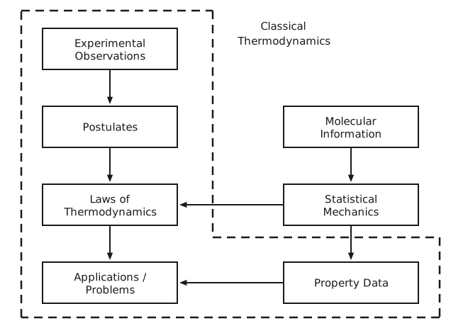
Figure 1. Scope of classical thermodynamics. A dashed boundary labelled “Classical Thermodynamics” encloses five boxes: Experimental Observations, Postulates, Laws of Thermodynamics, Applications / Problems, and Property Data. Inside that boundary the flow runs downward: Experimental Observations → Postulates → Laws of Thermodynamics → Applications / Problems. Outside the boundary, Molecular Information → Statistical Mechanics. Statistical Mechanics feeds two things across the boundary: an arrow left into Laws of Thermodynamics, and an arrow down into Property Data. Property Data in turn feeds an arrow left into Applications / Problems.
System and environment
System: things that are under study or analysis; e.g., a collection of matter, region of space, etc. Also called control volume.
Environment: everything else other than the system. Also called surroundings.
Boundary: imaginary or physical boundary that separates the system from its environment.
Universe: System + Environment.
Properties: attributes or characteristics of the system. Primitive properties are those that can be measured in a well-defined experiment. Derived properties are those that cannot be measured directly but nevertheless can be used to describe the system.
Types of systems
System interacts with its surroundings via the boundary, and is classified according to the types of interactions allowed.
Closed / open system: whether or not the boundary is impermeable to mass flow.
Movable / rigid boundary: whether or not the boundary can be displaced and mechanical work interactions can take place.
Adiabatic / diathermal: whether the boundary is a perfect heat insulator or conductor.
Isolated systems are ones with no interactions with the environment (i.e., closed adiabatic with rigid boundary). Universe is by definition isolated.
We also distinguish between simple and composite systems. The former is one without internal boundaries and not acted upon by external fields, while the latter consists of two or more simple systems. Simple systems can include multiple phases.
Restraints are barriers within a system that prevent some changes from occurring within the time span of interest; e.g., chemical reaction barriers, nucleation barriers. Internal boundaries are also restraints.
Reservoir is used for a system much larger than the system under study such that interactions between the two leave reservoir unchanged. Examples include large bodies of water, atmosphere, or any system with much larger mass than the mass of the system under study.
Stable equilibrium states
Postulate I (Duhem’s theorem)
For closed simple systems with given internal restraints, stable equilibrium states can be characterized completely by two independently variable properties in addition to the masses of the constituent chemical species.
Equilibrium states of a system are completely specified by \(E\) (or \(U\) when we do not care about \(E_{\mathrm{K}}\) and \(E_{\mathrm{P}}\)) and \(\vec{x}\). In fact, we will later postulate the existence of entropy \(S\), which is maximized at equilibrium states.
for an \(N\)-component system where there is only \(P \mathrm{d}V\) work.
Postulate II
In processes for which there is no net effect on the environment, all systems (simple and composite) with given internal restraints will approach one and only one stable equilibrium state for each simple subsystem. In the limiting condition, the entire system is said to be at equilibrium.
How do we know that the system is at equilibrium?
Never completely sure.
System independent of time.
System independent of history.
No energy or mass flow.
Rely on thermodynamic consistency check (e.g., using equilibrium criteria that we will develop later).
The state of a system consisting of \(N\) particles can be specified (in the classical picture) by the \(3N\) position coordinates \(\left(x_{1}, y_{1}, z_{1}, x_{2}, y_{2}, z_{2}, \dots, x_{N}, y_{N}, z_{N}\right)\) and the \(3N\) momentum coordinates \(\left(p_{x1}, p_{y1}, p_{z1}, p_{x2}, p_{y2}, p_{z2}, \dots, p_{xN}, p_{yN}, p_{zN}\right)\). \(N\) ~ \(10^{23}\) is a very large number. Equilibrium states can be characterized by a small number of macroscopic variables, such as \(P, T, ρ, M\).
From the mechanical definition of work to energy and heat
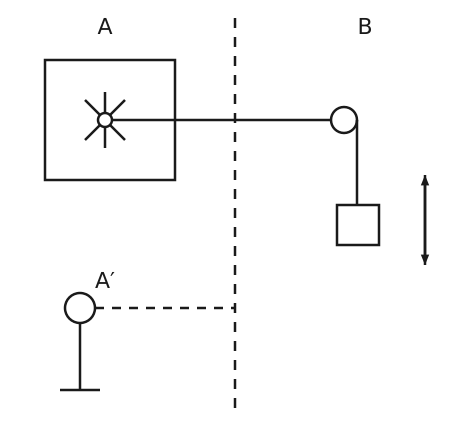
Figure 2. Adiabatic work interaction between systems A and B. A vertical dashed line marks the boundary. On the left, system A is a closed box containing a paddle wheel. A cord runs from the paddle-wheel shaft, crosses the boundary, passes over a pulley, and descends to a hanging weight on the right in system \(B\); a double-headed vertical arrow beside the weight indicates that it can rise or fall. Below, a second left-hand arrangement labelled A′ is sketched as a stick figure connected to the boundary by a dashed line, illustrating the point in step 2 that whatever lies outside A and \(B\) can be replaced by a mechanical device without changing what happens in A and \(B\).
Mechanical definition of work.
\[δw = \vec{F} \cdot \mathrm{d}\vec{x}\]That is, the differential work equals the dot product of the force vector with the differential displacement vector.
Adiabatic work interaction. (Parts external to A and \(B\) can be replaced by a mechanical device while causing the same changes in A and \(B\).) See Figure 2.
Postulate III defines energy.
\[E_{i} - E_{0} = W_{0\to i}^{\text{adiabatic}}\]That is, the energy difference between state \(i\) and reference state 0 equals the adiabatic work for the change from state 0 to state \(i\). See Figure 3.
\(ΔE = W + Q\) defines heat.
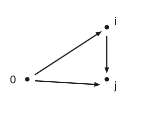
Figure 3. Adiabatic paths among states. Three points are marked: reference state 0 at the lower left, state \(i\) at the upper right, and state \(j\) at the lower right. Arrows run from 0 to \(i\), from 0 to \(j\), and from \(i\) to \(j\).
Postulate III
For any states (1) and (2), in which a closed system is at equilibrium, the change of state represented by (1) → (2) and/or the reverse change (2) → (1) can occur by at least one adiabatic process and the adiabatic work interaction between this system and its surroundings is determined uniquely by specifying the end states (1) and (2).
Postulate IV (Zeroth Law of Thermodynamics)
If the sets of systems A–\(B\) and A–\(C\) each have no heat interactions when connected across nonadiabatic walls, there will be no heat interaction if systems \(B\) and \(C\) are also connected.
If thermometric temperature \(θ_{A} < θ_{B}\), then energy is transferred from \(B\) to A, such that both of the following hold:
\(\mathrm{d}E_{B} < 0\)
\(\mathrm{d}E_{A} > 0\)
In other words, we require that the partial derivative of energy with respect to thermometric temperature be positive: