First Law of Thermodynamics

ChE 621 — Thermodynamics

Energy and the first law

From Postulate III (existence, additivity, and conservation), stated in full in the Introduction notes: There exists an extensive property called energy, \(E\). Energy is conserved for an isolated system. The energy of a system can only be changed via work or heat interactions with the environment.

\[\text{First law: } \mathrm{d}E = δQ + δW\]

• \(\mathrm{d}E\) is an exact differential, so its integral is independent of path and \(E\) is a state function:

  \[ΔE = \int_{E_{1}}^{E_{2}} \mathrm{d}E = E_{2} - E_{1}\]

• \(δQ\) and \(δW\) are inexact differentials, so their integrals are path dependent and \(Q\) and \(W\) are not state functions. We may write \(Q = \int δQ\) along the path from state 1 to state 2, but there is no such thing as \(ΔQ = Q_{2} - Q_{1}\).

Generalized work

\[\text{Generalized work }: δW = \vec{F} \cdot \mathrm{d}\vec{x}\]

• \(\vec{F}\) is the generalized force.

• \(\vec{x}\) is the generalized displacement.

Types of work	\(\vec{F} \cdot \mathrm{d}\vec{x}\)
Pressure–volume	\(- P \mathrm{d}V\)
Surface deformation	\(σ_{\mathrm{s}} \mathrm{d}\)a
Electric polarization	\(V\vec{E} \cdot \mathrm{d}\vec{D}\)
Magnetic polarization	\(V\vec{H} \cdot \mathrm{d}\vec{B}\)
Stress–strain	\(Vσ_{x} \mathrm{d}ϵ_{x}\)
Chemical	\(μ_{i} \mathrm{d}n_{i}\)

Electric and magnetic polarization work

The electric displacement field, or induction, is \(\mathbf{D} = ε_{0}\mathbf{E} + \mathbf{P}\). For the magnetic case, \(\mathbf{B}\) is the magnetic flux density and \(\mathbf{H}\) is the magnetic field strength, with \(\mathbf{H} = \frac{\mathbf{B}}{μ_{0}} - \mathbf{M}\).

Since \(\mathbf{B} = μ_{0}\left(\mathbf{H} + \mathbf{M}\right)\), we have

\[δW = Vμ_{0}\mathbf{H} \cdot \mathrm{d}\mathbf{H} + Vμ_{0}\mathbf{H} \cdot \mathrm{d}\mathbf{M}\]

This is the work needed to magnetize a material occupying volume \(V\). The first term exists even in vacuum, and the second term is what accounts for the magnetization of the material. In the context of the first law, if our system is the material, so that \(\mathrm{d}U\) does not include vacuum field energy, the second term is what should be used. Similarly, \(Vε_{0}\mathbf{E}\) d\(\mathbf{P}\) is what should be used for electric polarization.

Internal energy

\(E\) is usually separated into three parts for convenience:

\[\mathrm{d}E = \mathrm{d}U + \mathrm{d}E_{\mathrm{K}} + \mathrm{d}E_{\mathrm{P}}\]

• \(U\): internal energy associated with internal microscopic degrees of freedom (center-of-mass translation, rigid-body rotation, vibrations, and so on).

• \(E_{\mathrm{K}}\): kinetic energy associated with translational motion of the entire system.

• \(E_{\mathrm{P}}\): potential energy associated with an external field, for example gravity.

Heat

Heat is all the remaining modes of energy transfer that cannot be expressed as \(\vec{F} \cdot \mathrm{d}\vec{x}\). Consider two systems separated by a diathermal wall. The total system is isolated and the walls are rigid. Suppose A and \(B\) undergo an interaction that causes a change in their properties.

\[ΔE = ΔE_{A} + ΔE_{B} = Q_{A} + Q_{B} = 0\]

\[Q_{A} = - Q_{B} \text{ and } ΔE_{A} = - ΔE_{B}\]

When \(ΔE_{A} < 0\) and \(ΔE_{B} > 0\), we say energy is transferred from A to \(B\) in the form of heat, and vice versa.

Heat transfer results from microscopic work interactions that allow energy transfer between the system and its environment. We know intuitively that if A is hotter than \(B\), molecules in A are moving faster than those in \(B\), and the collisions between A molecules and wall atoms, and between wall atoms and \(B\) molecules, transfer microscopic momentum and kinetic energy from A to \(B\). The net result of many such collisions is heat transfer. Heat transfer is due to random, microscopic work done by constituent particles of one system on the other.

Reversibility

Definitions

A process is reversible if a second process could be performed so that both the system and its environment can be restored to their initial states, except for differential changes of second order.

A process is irreversible if changes in the system cannot be reversed in their entirety without making changes elsewhere in the universe.

A path is quasi-static if all the intermediate states are equilibrium states. All reversible processes are quasi-static, but the reverse is not necessarily true.

A process is internally reversible if it can be performed with an environment such that the system and all elements of this environment can be restored to their initial states, except for differential changes of second order in external work reservoirs.

Worked example: expansion of a gas against a weighted piston

Let us look at an example to illustrate the characteristics of a reversible process. A piston-cylinder system initially has a weight, \(m\), to keep the gas at pressure \(P_{\mathrm{i}}\). Removing the weight causes the gas to expand to a final pressure \(P_{\mathrm{f}} = P_{0}\).

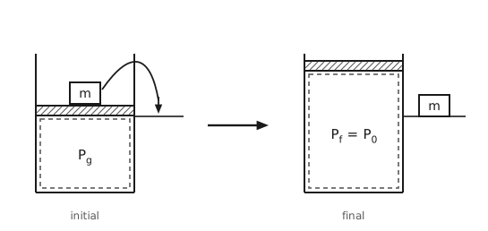
Figure 1. Expansion of a gas when the whole weight is removed at once. Two states side by side. On the left, the initial state: an open-topped cylinder holds a gas at pressure \(P_{\mathrm{g}}\), closed by a piston that carries a single weight labelled \(m\). A curved arrow runs from the weight, up over the cylinder wall, and down onto a ledge at the side. On the right, the final state: the piston has risen to the top of the cylinder, the enclosed gas is now at \(P_{\mathrm{f}} = P_{0}\), and the weight \(m\) rests on the ledge beside the cylinder.

If we choose the gas as the system, the work done is

\[\mathrm{d}W_{\mathrm{g}} = - P_{\mathrm{g}} \mathrm{d}V_{\mathrm{g}}\]

To evaluate \(P_{\mathrm{g}}\) we need the motion of the piston. Writing the acceleration in terms of the piston velocity \(v\) and its position \(z\),

\[m_{\mathrm{p}}a = m_{\mathrm{p}} \frac{\mathrm{d}^{2}z}{\mathrm{d}t^{2}} = m_{\mathrm{p}} \left(\frac{\mathrm{d}}{\mathrm{d}t}\right)\left(\frac{\mathrm{d}z}{\mathrm{d}t}\right)\]

and using the chain rule \(\frac{\mathrm{d}}{\mathrm{d}t} = \left(\frac{\mathrm{d}z}{\mathrm{d}t}\right)\left(\frac{\mathrm{d}}{\mathrm{d}z}\right)\), this becomes

\[m_{\mathrm{p}}a = m_{\mathrm{p}} v \frac{\mathrm{d}v}{\mathrm{d}z}\]

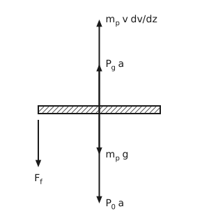
Figure 2. Free-body diagram of the piston. A hatched horizontal slab represents the piston. Four of the five forces are drawn on one vertical line through the centre of the piston. Two point upward from it: the longer is labelled \(m_{\mathrm{p}} v \frac{\mathrm{d}v}{\mathrm{d}z}\), the shorter \(P_{\mathrm{g}}\) a. Two point downward from it: the shorter is labelled \(m_{\mathrm{p}} g\), the longer \(P_{0}\) a. The fifth, friction \(F_{\mathrm{f}}\), acts at the wall and so is drawn downward from the left-hand edge of the piston.

Force balance to evaluate \(P_{\mathrm{g}}\):

\[P_{\mathrm{g}}a - P_{0}a - F_{\mathrm{f}} - m_{\mathrm{p}}g - m_{\mathrm{p}}v \frac{\mathrm{d}v}{\mathrm{d}z} = 0\]

Substituting back into the expression for the work gives

\[\mathrm{d}W_{\mathrm{g}} = - \left(P_{0} \mathrm{d}V_{\mathrm{g}} + m_{\mathrm{p}}g \mathrm{d}z + m_{\mathrm{p}}v \mathrm{d}v + F_{\mathrm{f}} \mathrm{d}z\right)\]

These four terms are:

• \(P_{0} \mathrm{d}V_{\mathrm{g}}\) is the work of pushing against the atmosphere.

• \(m_{\mathrm{p}}g \mathrm{d}z\) and \(m_{\mathrm{p}}v \mathrm{d}v\) together are the gravitational and acceleration terms for the piston.

• \(F_{\mathrm{f}} \mathrm{d}z\) is the dissipative loss.

Expansion in one step

Even if we ignore the mass of the piston \(\left(m_{\mathrm{p}} = 0\right)\) and friction \(\left(F_{\mathrm{f}} = 0\right)\), the work done is

\[W_{\mathrm{g}} = - \int_{V_{\mathrm{i}}}^{V_{\mathrm{f}}} P_{0} \mathrm{d}V_{\mathrm{g}} = - P_{0}\left(V_{\mathrm{f}} - V_{\mathrm{i}}\right)\]

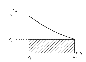
Figure 3. Pressure–volume diagram for the single-step expansion. Pressure is on the vertical axis and volume on the horizontal axis. A curve falls from \(P_{\mathrm{i}}\) at \(V_{\mathrm{i}}\) to \(P_{0}\) at \(V_{\mathrm{f}}\). Dashed guide lines mark \(P_{\mathrm{i}}, P_{0}, V_{\mathrm{i}}\) and \(V_{\mathrm{f}}\). The hatched rectangle beneath the curve, of height \(P_{0}\) and width \(V_{\mathrm{f}} - V_{\mathrm{i}}\), is the work actually done by the gas against the constant external pressure. The area between that rectangle and the curve is the work that is not recovered.

In order to reverse the process, the weight must be lifted back through the height it fell:

\[W_{\text{rev}} = mg\left(z_{2} - z_{1}\right)\]

Expansion in two steps

Now consider the same end states achieved in more steps.

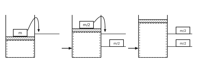
Figure 4. The same expansion carried out in two half steps. Three panels in sequence. In the first, the piston carries the whole weight \(m\). In the second, half the weight has been slid off onto a ledge, the gas has expanded, and the piston now carries a weight \(\frac{m}{2}\) with one \(\frac{m}{2}\) resting on the ledge. In the third, the second half has also been removed, the piston has risen to the top, and both \(\frac{m}{2}\) weights rest on ledges beside the cylinder. Arrows between the panels show the order, and within the first two panels a curved arrow runs from the weight on the piston, over the cylinder wall, to the ledge the next half is about to be set down on.

\[W_{\text{rev}} = \left(\frac{m}{2}\right)\left(z_{2} - z_{1}\right)g\]

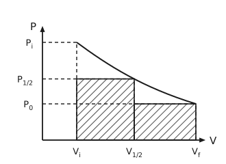
Figure 5. Pressure–volume diagram for the two-step expansion. The same falling curve as before, now with three pressure levels marked, \(P_{\mathrm{i}}, P_{1/2}\) and \(P_{0}\), and three volumes, \(V_{\mathrm{i}}, V_{1/2}\) and \(V_{\mathrm{f}}\). Two hatched rectangles sit beneath the curve: the first spans \(V_{\mathrm{i}}\) to \(V_{1/2}\) at height \(P_{1/2}\), the second spans \(V_{1/2}\) to \(V_{\mathrm{f}}\) at height \(P_{0}\). Together they cover more of the area under the curve than the single rectangle of Figure 3.

Expansion in many steps, and the reversible limit

\[W_{\text{rev}} = \left(\frac{m}{N}\right)\left(z_{2} - z_{1}\right)g\]

\[\text{As } N \to \infty, W_{\text{rev}} \to 0\]

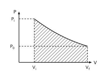
Figure 6. Pressure–volume diagram in the many-step limit. The same falling curve, with \(P_{\mathrm{i}}\) and \(P_{0}\) marked on the vertical axis and \(V_{\mathrm{i}}\) and \(V_{\mathrm{f}}\) on the horizontal axis. The hatched region now fills the whole area under the curve between \(V_{\mathrm{i}}\) and \(V_{\mathrm{f}}\), because in the limit of infinitely many infinitesimal steps the staircase of rectangles becomes the curve itself.

The reversible process is an idealization that proceeds at an infinitesimal rate and takes an infinite amount of time. The system never leaves equilibrium, that is, it is quasi-static.

Mathematical relations of functions of state

This section follows Tester & Modell, Appendix B.

Inexact differentials

Consider the line integral that defines work, which is path dependent:

\[W = \vec{F} \cdot Δ\vec{x} \to δW = \vec{F}\left(\vec{x}\right) \cdot \mathrm{d}\vec{x}\]

\[W = \int_{C} δw = \int_{C} \vec{F} \cdot \mathrm{d}\vec{x}\]

where \(C\) is the path followed from state 1 to state 2.

Differentials like these are inexact differentials.

Exact differentials

An exact differential is the total derivative of some scalar function. The line integral of an exact differential is path independent and equals the difference of the scalar function evaluated at the end points.

Consider

\[M\left(x,y,z\right) \mathrm{d}x + N\left(x,y,z\right) \mathrm{d}y + P\left(x,y,z\right) \mathrm{d}z\]

The above differential is exact if and only if all three of the following hold:

\[\left(\frac{\partial M}{\partial y}\right)_{xz} = \left(\frac{\partial N}{\partial x}\right)_{yz}\]

\[\left(\frac{\partial M}{\partial z}\right)_{xy} = \left(\frac{\partial P}{\partial x}\right)_{yz}\]

\[\left(\frac{\partial N}{\partial z}\right)_{xy} = \left(\frac{\partial P}{\partial y}\right)_{xz}\]

Being an exact differential means that one can find a scalar function \(f\left(x,y,z\right)\) such that

\[\mathrm{d}f\left(x,y,z\right) = \left(\frac{\partial f}{\partial x}\right)_{yz} \mathrm{d}x + \left(\frac{\partial f}{\partial y}\right)_{xz} \mathrm{d}y + \left(\frac{\partial f}{\partial z}\right)_{xy} \mathrm{d}z\]

\[\equiv M\left(x,y,z\right) \mathrm{d}x + N\left(x,y,z\right) \mathrm{d}y + P\left(x,y,z\right) \mathrm{d}z\]

Term by term, \(\left(\frac{\partial f}{\partial x}\right)_{yz} = M, \left(\frac{\partial f}{\partial y}\right)_{xz} = N\), and \(\left(\frac{\partial f}{\partial z}\right)_{xy} = P\).

The scalar function is the multivariate analogue of the indefinite integral. The vector field formed by \(\left(M, N, P\right)\) is called conservative. Examples of conservative vector fields include forces that are gradients of some scalar functions that are the corresponding potentials, such as the gravitational potential and the electrostatic potential.

Heat capacities

Heat capacity is a material property that measures how much the material needs to increase in \(T\) to accommodate a certain amount of pure heat interactions (no work). Under constant \(V\):

\[C_{V} = \frac{δQ}{\mathrm{d}T} = \left(\frac{\mathrm{d}U}{\mathrm{d}T}\right)_{V}\]

\(C_{V}\) is extensive and is a function of \(T\). Specific heat capacities can be defined on either a per-mole or a per-mass basis:

\[\hat{C}_{V} = \left(\frac{\mathrm{d}\hat{U}}{\mathrm{d}T}\right)_{V} \text{ and } \tilde{C}_{V} = \left(\frac{\mathrm{d}\tilde{U}}{\mathrm{d}T}\right)_{V}\]

with \(\hat{U} = \frac{U}{m}\) and \(\tilde{U} = \frac{U}{n}\). Under constant \(P\):

\[\hat{C}_{P} = \left(\frac{\mathrm{d}\hat{H}}{\mathrm{d}T}\right)_{P} \text{ and } \tilde{C}_{P} = \left(\frac{\mathrm{d}\tilde{H}}{\mathrm{d}T}\right)_{P}\]

where \(H\) is the enthalpy, to be discussed later.

Ideal gases

Ideal gases are systems that satisfy the ideal gas law:

\[PV = nRT \text{ or } P\tilde{V} = RT\]

The assumptions are (1) no intermolecular interactions and (2) particles with no excluded volume.

\[\tilde{C}_{V} = \frac{3}{2}R, \tilde{C}_{P} = \frac{5}{2}R \text{ for monatomic gases }\]

\[\tilde{C}_{V} = \frac{5}{2}R, \tilde{C}_{P} = \frac{7}{2}R \text{ for diatomic gases }\]

\[\frac{\tilde{C}_{P}}{R} = A + BT + CT^{2} + \frac{D}{T^{2}} \text{ for temperature-dependent heat capacities }\]

First law for open systems

We want to derive a relationship between \(\mathrm{d}E_{Ω} = E_{Ω2} - E_{Ω1}\) and the heat and work interactions at the open system boundary.

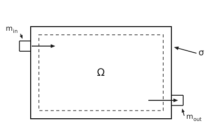
Figure 7. Open system, or control volume. A solid rectangle encloses a dashed region labelled Ω. A short duct enters through the upper left of the solid boundary, with an arrow showing mass \(m_{\text{in}}\) flowing in. A second duct leaves through the lower right, with an arrow showing mass \(m_{\text{out}}\) flowing out. A label \(σ\) with a leader line points at the solid boundary, which is the surface across which heat and work cross.

The combination \(Ω + \mathrm{d}m_{\text{in}} + \mathrm{d}m_{\text{out}}\) forms a closed system.

State 1, at time \(t_{1}\):

\[E_{1} = E_{Ω1} + \hat{E}_{\text{in}} \cdot \mathrm{d}m_{\text{in}}\]

State 2, at time \(t_{2}\):

\[E_{2} = E_{Ω2} + \hat{E}_{\text{out}} \cdot \mathrm{d}m_{\text{out}}\]

Subtracting,

\[\mathrm{d}E = E_{2} - E_{1} = \mathrm{d}E_{Ω} + \hat{E}_{\text{out}} \cdot \mathrm{d}m_{\text{out}} - \hat{E}_{\text{in}} \cdot \mathrm{d}m_{\text{in}}\]

The work splits into the work done across \(σ\) and the flow work needed to push the mass across the boundary:

\[δW = δW_{σ} + P_{\text{in}} \cdot \mathrm{d}V_{\text{in}} - P_{\text{out}} \cdot \mathrm{d}V_{\text{out}}\]

\[= δW_{σ} + P_{\text{in}} \cdot \hat{V}_{\text{in}} \cdot \mathrm{d}m_{\text{in}} - P_{\text{out}} \cdot \hat{V}_{\text{out}} \cdot \mathrm{d}m_{\text{out}}\]

Since all the heat crosses \(σ\),

\[\mathrm{d}E = δW + δQ = δW + δQ_{σ}\]

Combining these gives the open-system energy balance:

\[\mathrm{d}E_{Ω} = δQ_{σ} + δW_{σ} + \left(\hat{E}_{\text{in}} + P_{\text{in}} \cdot \hat{V}_{\text{in}}\right) \cdot \mathrm{d}m_{\text{in}} - \left(\hat{E}_{\text{out}} + P_{\text{out}} \cdot \hat{V}_{\text{out}}\right) \cdot \mathrm{d}m_{\text{out}}\]

The grouped terms are the enthalpy per unit mass, and the specific energy carried by the stream:

\[\hat{H} \equiv \hat{U} + P\hat{V} \text{ and } \hat{E}_{\text{in}/\text{out}} = \hat{U}_{\text{in}/\text{out}} + \tfrac{1}{2} v^{2}_{\text{in}/\text{out}} + gz_{\text{in}/\text{out}}\]

Generalizing to any number of streams,

\[\mathrm{d}E_{Ω} = δQ_{σ} + δW_{σ} + \sum _{i} \left(\hat{H}_{i} + \tfrac{1}{2} v_{i}^{2} + gz_{i}\right) ξ_{i} \cdot \mathrm{d}m_{i}\]

where the sign factor \(ξ_{i}\) is +1 for an inlet and −1 for an outlet.

Typically, for Ω at rest and with gravitational potential energy being negligible, we have

\[\mathrm{d}U_{Ω} = δQ_{σ} + δW_{σ} + \sum _{i} \hat{H}_{i} ξ_{i} \cdot \mathrm{d}m_{i}\]

Rate form

We can integrate these equations between two states, or differentiate them to obtain the temporal evolution of the system through a set of equilibrium states:

\[\dot{U}_{Ω} = \dot{Q}_{σ} + \dot{W}_{σ} + \sum _{i} \left(\hat{H}_{i} + \tfrac{1}{2} v_{i}^{2} + gz_{i}\right) ξ_{i} \cdot \dot{m}_{i}\]

• \(\dot{Q}_{σ} = \frac{δQ}{\mathrm{d}t}\) is the rate of heat transfer across \(σ\).

• \(\dot{W}_{σ} = \frac{δW_{σ}}{\mathrm{d}t}\) is the power of work across \(σ\).

• \(\dot{m}_{i} = \frac{\mathrm{d}m_{i}}{\mathrm{d}t} = ρ_{i}\)a\(_{i}v_{i}\) is the rate of mass flow into or out of \(σ\).

The energy balance is often coupled to a material balance:

\[\mathrm{d}M_{Ω} = \sum _{i} ξ_{i} \cdot \mathrm{d}m_{i}\]

\[\dot{M}_{Ω} = \sum _{i} ξ_{i} \cdot \dot{m}_{i}\]

At steady state, time derivatives are zero for the accumulation terms, so \(\dot{U}_{Ω} = 0\) and \(\dot{M}_{Ω} = 0\).

Integral form for distributed variables

In cases where variables are distributed and vary along \(σ\), and \(E_{Ω}\) is not uniform within Ω, an integral form should be used:

\[\int_{Ω} \frac{\partial \left(\hat{ρ}\hat{E}\right)}{\partial t} \mathrm{d}V = - \int_{Ω} \dot{Q} \cdot \vec{n} \mathrm{d}A_{σ} + \sum _{i} \dot{W}_{σ,i} - \int_{σ} \hat{ρ}\left(\hat{H} + \frac{v^{2}}{2} + gz\right) \vec{v} \cdot \vec{n} \mathrm{d}A_{σ}\]

The region of integration on the middle term is written \(Ω\) in the original, although the area element beside it is \(\mathrm{d}A_{σ}\). It is transcribed as written.

Closed systems at steady state

Problem

Compression of an ideal gas (with \(C_{V}, C_{P}\)) in a piston-cylinder from \(P_{1}, V_{1}, T_{1}\) to \(P_{2}, V_{2}, T_{2}\). When the piston reaches \(V_{2}\), it is latched in place. Now suppose we are interested in the gas temperature: what is the highest \(T_{2}\) the gas will rise to?

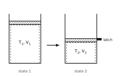
Figure 8. Compression of an ideal gas, with the piston then latched. Two states side by side. In state 1 the piston sits high in the cylinder and the gas occupies a large dashed region labelled \(T_{1}, V_{1}\). An arrow leads to state 2, where the piston has been pushed down, the gas occupies a smaller dashed region labelled \(T_{2}, V_{2}\), and a solid block on the cylinder wall marks the latch that holds the piston in place.

From the ideal gas law,

\[pV = nRT\]

\[\frac{P_{1}V_{1}}{P_{2}V_{2}} = \frac{T_{1}}{T_{2}}\]

leads no where. The energy balance for the closed system is

\[\mathrm{d}U = δQ + δW\]

Scenario I: reversible and isothermal

\[\mathrm{d}U = δQ + δW\]

\[W = \int_{V_{1}}^{V_{2}} - P \mathrm{d}V = - \int_{V_{1}}^{V_{2}} \left(\frac{nRT}{V}\right) \mathrm{d}V = - nRT_{0} \ln \left(\frac{V_{2}}{V_{1}}\right)\]

Here \(T_{0}\) is the constant temperature at which the isothermal compression is carried out.

Scenario II: reversible and adiabatic

With no heat interaction, \(\mathrm{d}U = δW\), so

\[n\tilde{C}_{V} \mathrm{d}T = - P \mathrm{d}V = - \left(\frac{nRT}{V}\right) \mathrm{d}V\]

Separating variables and integrating,

\[\int_{T_{1}}^{T_{2}} \frac{\mathrm{d}T}{T} = - \left(\frac{R}{\tilde{C}_{V}}\right) \int_{V_{1}}^{V_{2}} \frac{\mathrm{d}V}{V}\]

\[\ln \left(\frac{T_{2}}{T_{1}}\right) = - \left(\frac{R}{\tilde{C}_{V}}\right) \ln \left(\frac{V_{2}}{V_{1}}\right)\]

\[\frac{T_{2}}{T_{1}} = \left(\frac{V_{2}}{V_{1}}\right)^{- R/\tilde{C}_{V}}\]

Introducing the heat capacity ratio \(γ \equiv \frac{\tilde{C}_{P}}{\tilde{C}_{V}}\) and using \(R = \tilde{C}_{P} - \tilde{C}_{V}\), this becomes

\[\frac{T_{2}}{T_{1}} = \left(\frac{V_{2}}{V_{1}}\right)^{1- γ}\]

\[\frac{T_{2}}{T_{1}} = \left(\frac{P_{1}}{P_{2}}\right)^{\left(1- γ\right)/γ} = \left(\frac{P_{2}}{P_{1}}\right)^{R/\tilde{C}_{P}}\]

\[P_{1}V_{1}^{γ} = P_{2}V_{2}^{γ}\]

Closed systems at non-steady state

• For non-steady state problems, we are usually interested in how the properties of the system evolve with time.

• For example, consider what happens to the temperature of the gas and the cylinder as a function of time after the adiabatic compression (Scenario II).

Define two systems:

• System A: the gas, at temperature \(T_{\mathrm{g}}\).

• System \(B\): the cylinder and piston, which have mass, at temperature \(T_{\mathrm{w}}\).

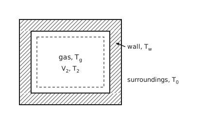
Figure 9. Gas, cylinder wall, and surroundings. A hatched band forms the cylinder wall, which is system \(B\) at temperature \(T_{\mathrm{w}}\). Inside it a dashed region holds the gas, system A, at temperature \(T_{\mathrm{g}}\), occupying \(V_{2}\) at \(T_{2}\) immediately after the compression. Outside the wall are the surroundings, held at \(T_{0}\). Heat passes from the gas to the wall, and from the wall to the surroundings.

\[\frac{\mathrm{d}U_{A}}{\mathrm{d}t} = - hA\left(T_{\mathrm{g}} - T_{\mathrm{w}}\right)\]

\[\frac{\mathrm{d}U_{B}}{\mathrm{d}t} = hA\left(T_{\mathrm{g}} - T_{\mathrm{w}}\right) - hA\left(T_{\mathrm{w}} - T_{0}\right)\]

Writing the internal energies in terms of heat capacities,

\[n\tilde{C}_{V,\mathrm{g}} \dot{T}_{\mathrm{g}} = - hA\left(T_{\mathrm{g}} - T_{\mathrm{w}}\right)\]

\[m\hat{C}_{V,\mathrm{w}} \dot{T}_{\mathrm{w}} = hA\left(T_{\mathrm{g}} - T_{\mathrm{w}}\right) - hA\left(T_{\mathrm{w}} - T_{0}\right)\]

The original writes this pair as a single matrix equation for the state vector \(\left(T_{\mathrm{g}}, T_{\mathrm{w}}\right)\):

\[\begin{split}\frac{\mathrm{d}}{\mathrm{d}t} \begin{pmatrix} T_{\mathrm{g}} \\ T_{\mathrm{w}} \end{pmatrix} = \begin{pmatrix} - \dfrac{hA}{n\tilde{C}_{V\mathrm{g}}} & \dfrac{hA}{n\tilde{C}_{V\mathrm{g}}} \\[8pt] \dfrac{hA}{m\hat{C}_{V,\mathrm{w}}} & - \dfrac{2hA}{m\hat{C}_{V,\mathrm{w}}} \end{pmatrix} \begin{pmatrix} T_{\mathrm{g}} \\ T_{\mathrm{w}} \end{pmatrix} + \begin{pmatrix} 0 \\[8pt] \dfrac{hAT_{0}}{m\hat{C}_{V,\mathrm{w}}} \end{pmatrix}\end{split}\]

that is, \(\frac{\mathrm{d}}{\mathrm{d}t}\vec{T} = \mathbf{A}\vec{T} + \mathbf{b}\) for the state vector \(\vec{T} = \left(T_{\mathrm{g}}, T_{\mathrm{w}}\right)\).

Limiting case I: large wall mass

As \(m \to \infty\),

\[\dot{T}_{\mathrm{w}} = \frac{hA}{m\hat{C}_{V,\mathrm{w}}} \left[\left(T_{\mathrm{g}} - T_{\mathrm{w}}\right) - \left(T_{\mathrm{w}} - T_{0}\right)\right] \to 0\]

\[T_{\mathrm{w}} = T_{0}\]

so the wall acts as a reservoir and the gas equation becomes

\[n\tilde{C}_{V,\mathrm{g}} \dot{T}_{\mathrm{g}} = - hA\left(T_{\mathrm{g}} - T_{0}\right)\]

\[\ln \left[\frac{T - T_{0}}{T_{2} - T_{0}}\right] = \frac{- hAt}{n\tilde{C}_{V\mathrm{g}}}\]

so that

• \(T = T_{2}\) at \(t = 0\);

• \(T \to T_{0}\) as \(t \to \infty\).

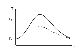
Figure 10. Sketch of temperature against time. Time runs along the horizontal axis and temperature up the vertical axis, with \(T_{2}\) and \(T_{0}\) marked. A solid curve rises from near \(T_{0}\) to a peak slightly above \(T_{2}\) and then decays back towards \(T_{0}\). A dashed curve leaves the peak and decays towards \(T_{0}\) alongside it, at half the height of the solid curve above \(T_{0}\) at every instant. A horizontal dashed line marks the \(T_{0}\) asymptote and a vertical dashed line the time of the peak. Neither curve is labelled in the original.

Limiting case II: negligible wall heat capacity

As \(m\hat{C}_{V,\mathrm{w}} \to 0\),

\[hA\left(T_{\mathrm{g}} - T_{\mathrm{w}}\right) - hA\left(T_{\mathrm{w}} - T_{0}\right) = m\hat{C}_{V,\mathrm{w}} \dot{T}_{\mathrm{w}} \to 0\]

\[T_{\mathrm{w}} = \frac{T_{\mathrm{g}} + T_{0}}{2}\]

so the wall temperature simply sits halfway between the gas and the surroundings, and

\[n\tilde{C}_{V,\mathrm{g}} \dot{T}_{\mathrm{g}} = - \left(\frac{hA}{2}\right)\left(T_{\mathrm{g}} - T_{0}\right)\]

\[T = T_{0} + \left(T_{2} - T_{0}\right) \cdot \mathrm{e}^{- hAt/\left(2n\tilde{C}_{V\mathrm{g}}\right)}\]

Open systems at steady state

Problem

A cylindrical steel rod (radius \(r = 0.1\) m, \(ρ = 7833\) kg/m\(^{3}\), and \(C_{P} = 0.465\) kJ/kg·K) is treated continuously by being drawn at \(v = 3\) m/min through a 6 m long furnace maintained at \(T = 900\) °C. At steady state operation the rod enters the furnace at \(T_{1} = 30\) °C and leaves at \(T_{2} = 700\) °C. The furnace is also cylindrical and has a diameter 10 times that of the rod. The coefficient of thermal expansion is negligible. Determine the rate of heat transfer to the rods in the furnace.

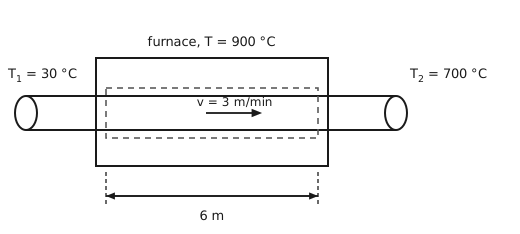
Figure 11. Steel rod drawn through the furnace. A long cylindrical rod passes horizontally through a rectangular furnace held at \(T = 900\) °C. The rod enters from the left at \(T_{1} = 30\) °C and leaves at the right at \(T_{2} = 700\) °C, drawn at \(v = 3\) m/min. A dashed rectangle around the length of rod inside the furnace marks the control volume, and a dimension arrow below marks the 6 m furnace length.

Starting from the rate form, with no shaft work across \(σ\),

\[\dot{U}_{Ω} = \dot{Q}_{σ} + \cancel{\dot{W}_{σ}} + \sum _{i} \left(\hat{H}_{i} + \tfrac{1}{2} v_{i}^{2} + gz_{i}\right) ξ_{i} \cdot \dot{m}_{i}\]

The material balance gives

\[\dot{M}_{Ω} = \dot{m}_{1} - \dot{m}_{2} = 0 \implies \dot{m}_{1} = \dot{m}_{2} = \dot{m}\]

At steady state the accumulation vanishes, and the kinetic and potential terms are negligible. Those terms are struck through below, as they are in the original:

\[\dot{U}_{Ω} = \dot{Q}_{σ} + \dot{m}\left[\left(\hat{H}_{1} + \cancel{\tfrac{1}{2} v_{1}^{2}} + \cancel{gz_{1}}\right) - \left(\hat{H}_{2} + \cancel{\tfrac{1}{2} v_{2}^{2}} + \cancel{gz_{2}}\right)\right] = 0\]

which leaves

\[\dot{Q}_{σ} = \dot{m}\hat{C}_{P}\left(T_{2} - T_{1}\right) = \hat{ρ}A \cdot v \hat{C}_{P}\left(T_{2} - T_{1}\right)\]

\[= 230,000 \text{ kJ/min } = 3833 \text{ kW }\]

Differential energy balances

Suppose that we are interested in another aspect of steel rod annealing, such as scaling it up, so we need the heat transfer coefficient

\[\dot{Q} = hAΔT\]

or we want to know how the temperature varies as the rod travels through the furnace.

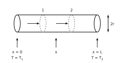
Figure 12. Differential element of the rod. The rod is drawn as a horizontal cylinder of diameter \(2r\). Two dashed cross-sections divide it, labelled 1 and 2, with arrows showing the direction of travel through each. Below the rod, three upward arrows mark positions along its axis: \(x = 0\) where \(T = T_{1}\), a general position \(x\), and \(x = L\) where \(T = T_{2}\).

Applying the steady-state balance to the element,

\[\dot{Q} = 2πr \cdot \mathrm{d}x \cdot h\left(T - T_{\mathrm{f}}\right)\]

\[\dot{U}_{Ω} = \dot{Q}_{σ} + \cancel{\dot{W}_{σ}} + \dot{m}_{1}\hat{H}_{1} - \dot{m}_{2}\hat{H}_{2} = 0\]

\[\dot{m}_{1} = \dot{m}_{2} = \dot{m} = \hat{ρ}πr^{2}v\]

so that

\[2πrh\left(T_{\mathrm{f}} - T\right) \mathrm{d}x = \hat{ρ}πr^{2}v\hat{C} \mathrm{d}T\]

Integrating along the rod,

\[x = \frac{\hat{ρ}rv\hat{C}}{2h} \ln \left[\frac{T_{1} - T_{\mathrm{f}}}{T - T_{\mathrm{f}}}\right]\]

\[T = T_{\mathrm{f}} + \left(T_{1} - T_{\mathrm{f}}\right) \cdot \mathrm{e}^{- 2hx/\left(\hat{ρ}rv\hat{C}\right)}\]

Open systems at non-steady state

Problem

An empty gas tank is filled from a constant source of ideal gas. What is the final \(T\) in the tank?

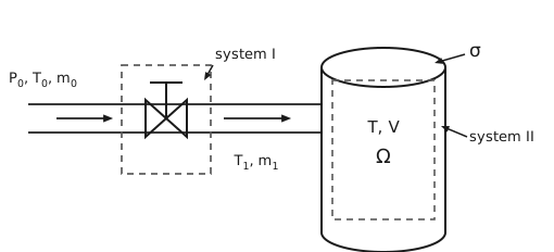
Figure 13. Filling an empty tank through a valve. Gas at \(P_{0}, T_{0}\) flows at rate \(m_{0}\) along a pipe from the left, through a valve, and on into a vertical cylindrical tank at the right. A dashed box around the valve marks system I. Downstream of the valve the stream is at \(T_{1}\) with rate \(m_{1}\). The tank interior is dashed and labelled Ω with contents at \(T, V\); the tank is system II, and its boundary is labelled \(σ\).

System I: the valve

The energy balance for the valve has no accumulation, no heat interaction and no shaft work, so

\[\cancel{\dot{U}_{Ω}} = \cancel{\dot{Q}_{σ}} + \cancel{\dot{W}_{σ}} + \sum _{i} \left(\hat{H}_{i} + \tfrac{1}{2} v_{i}^{2} + gz_{i}\right) ξ_{i} \cdot \dot{m}_{i}\]

\[\hat{H}_{0} \cdot \dot{m}_{0} = \hat{H}_{1} \cdot \dot{m}_{1}\]

and the mass balance gives \(\dot{m}_{0} = \dot{m}_{1}\). Together these imply

\[\hat{H}_{0} = \hat{H}_{1} \left(\text{ the valve is ``isenthalpic'' }\right), \text{ so } T_{0} = T_{1}\]

System II: the tank

For the tank there is no heat interaction and no shaft work, so only the inlet enthalpy term survives:

\[\dot{U}_{Ω} = \cancel{\dot{Q}_{σ}} + \cancel{\dot{W}_{σ}} + \sum _{i} \left(\hat{H}_{i} + \tfrac{1}{2} v_{i}^{2} + gz_{i}\right) ξ_{i} \cdot \dot{m}_{i}\]

\[\frac{\mathrm{d}U_{Ω}}{\mathrm{d}t} = \hat{H}_{1} \cdot \dot{m}_{1} = \tilde{H}_{1} \cdot \dot{n}_{1}\]

with the mass balance

\[\frac{\mathrm{d}M_{Ω}}{\mathrm{d}t} = \dot{m}_{1}, \text{ or } \frac{\mathrm{d}n_{Ω}}{\mathrm{d}t} = \dot{n}_{1}\]

Together these give

\[\mathrm{d}U_{Ω} = \tilde{H}_{1} \cdot \dot{n}_{1} \cdot \mathrm{d}t = \tilde{H}_{1} \cdot \mathrm{d}n_{Ω}\]

Integrate from \(t = 0\), where \(U_{Ω} = 0\) and \(n_{Ω} = 0\):

\[\int_{0}^{U_{Ω}} \mathrm{d}U_{Ω} = \tilde{H}_{1} \int_{0}^{n_{Ω}} \mathrm{d}n_{Ω}\]

\[U_{Ω} = \left(\tilde{U}_{1} + P_{1}\tilde{V}_{1}\right) n_{Ω}\]

\[\tilde{U}_{Ω} = \tilde{U}_{1} + P_{1}\tilde{V}_{1}\]

For an ideal gas, \(P_{1}\tilde{V}_{1} = RT_{1}\), so

\[\tilde{U}_{Ω} - \tilde{U}_{1} = \tilde{C}_{V}\left(T_{Ω} - T_{1}\right) = P_{1}\tilde{V}_{1} = RT_{1}\]

\[T_{Ω} = \left(1 + \frac{R}{\tilde{C}_{V}}\right) T_{1} = γT_{1} = γT_{0}\]

The final temperature in the tank is therefore \(γ\) times the temperature of the source.