Calculus of Thermodynamics

ChE 621 — Thermodynamics.

The fundamental property equation

The motivation for studying the calculus of thermodynamic functions is to calculate the state variables appearing in the first and second laws using experimentally measurable primitive properties such as \(P, V\), and \(T\). For example,

\[\mathrm{d}\tilde{U} = \left(\frac{\partial \tilde{U}}{\partial T}\right)_{V} \mathrm{d}T + \left(\frac{\partial \tilde{U}}{\partial V}\right)_{T} \mathrm{d}V, \text{ with } \left(\frac{\partial \tilde{U}}{\partial T}\right)_{V} = \tilde{C}_{V}\]
\[\mathrm{d}\tilde{H} = \left(\frac{\partial \tilde{H}}{\partial T}\right)_{P} \mathrm{d}T + \left(\frac{\partial \tilde{H}}{\partial P}\right)_{T} \mathrm{d}P, \text{ with } \left(\frac{\partial \tilde{H}}{\partial T}\right)_{P} = \tilde{C}_{P}\]

There is no prescription in the first and second laws on the other derivatives.

Entropy representation

\[S = S\left(U, V, n_{1}, n_{2}, \dots \right)\]
\[\mathrm{d}S = \left(\frac{\partial S}{\partial U}\right)_{\vec{x}} \mathrm{d}U + \sum _{i} \left(\frac{\partial S}{\partial x_{i}}\right)_{U,\, x_{j}} \mathrm{d}x_{i}\]

where \(x = V\), and so on. Substituting the reversible form of the first law,

The bracketed group is zero, which gives

\[\left(\frac{\partial S}{\partial x_{i}}\right)_{U,\, x_{j}} = -\frac{F_{i}}{T}\]

and therefore

\[\mathrm{d}S = \frac{\mathrm{d}U}{T} - \frac{1}{T} \sum F_{i} \cdot \mathrm{d}x_{i}\]

Integration of this equation gives \(S\left(U, x\right)\). This is therefore called the entropy representation of the states of the system.

Energy representation

Alternatively, the energy representation, \(U\left(S, V, N\right)\), for a system with \(N\) species, characterized by extensive variables \(V\) and \(S\):

\[\mathrm{d}U = T \mathrm{d}S + \sum _{i} F_{i} \mathrm{d}x_{i} + \sum _{i} μ_{i} \mathrm{d}n_{i}\]

Term by term,

\[\left(\frac{\partial U}{\partial S}\right)_{V,\, n_{i}} = T\]
\[\left(\frac{\partial U}{\partial n_{i}}\right)_{S,\, V,\, n_{j}} = μ_{i}\]
\[\left(\frac{\partial U}{\partial V}\right)_{S,\, n_{i}} = - P\]

Example: entropy representation for a monatomic ideal gas

The entropy representation of the fundamental equation for a monatomic ideal gas is

\[S = S_{0} + NR \ln \left[\left(\frac{U}{U_{0}}\right)^{3/2} \cdot \left(\frac{V}{V_{0}}\right)\right]\]

Per mole,

\[\tilde{S} = \frac{S}{N} = \tilde{S}_{0} + R \ln \left[\left(\frac{\tilde{U}}{\tilde{U}_{0}}\right)^{3/2} \left(\frac{\tilde{V}}{\tilde{V}_{0}}\right)\right]\]

Solving for \(\tilde{U}\):

\[\tilde{U} = \tilde{U}_{0} \left(\frac{\tilde{V}_{0}}{\tilde{V}}\right)^{2/3} \exp \left[\frac{2}{3}\,\frac{\tilde{S} - \tilde{S}_{0}}{R}\right]\]

\(U\left(S, V, N\right)\) has complete information about the ideal gas. For example, differentiate with respect to \(S\) to get \(T\):

\[T = \left(\frac{\partial \tilde{U}}{\partial \tilde{S}}\right)_{\tilde{V}} = \tilde{U} \cdot \frac{2}{3}\,\frac{1}{R} \implies \tilde{U} = \frac{3}{2} RT\]
\[\tilde{C}_{V} = \left(\frac{\partial \tilde{U}}{\partial T}\right)_{\tilde{V}} = \frac{3}{2} R\]

That is, \(U\left(S, V, N\right)\) contains information about the heat capacity.

Similarly, differentiate with respect to \(V\) to get \(P\):

\[- P = \left(\frac{\partial \tilde{U}}{\partial \tilde{V}}\right)_{\tilde{S}} = - \frac{2}{3} \cdot \frac{1}{\tilde{V}} \cdot \tilde{U} \implies P = \frac{2}{3} \cdot \frac{\tilde{U}}{\tilde{V}}\]
\[P\tilde{V} = RT, \text{ so } P = \frac{RT}{\tilde{V}}\]

That is, \(U\left(S, V, N\right)\) contains the ideal gas law. On the other hand, the \(P\)-\(V\)-\(T\) equation of state is incomplete: it does not have \(C_{V}\) data. The \(U\)-\(V\)-\(T\) equation of state is also incomplete: it does not have the \(P\)-\(V\)-\(T\) relationship.

\(U\left(S, V, N\right)\) is inconvenient to use, because its independent variable \(S\) is not directly measurable.

  • Are there other energy functions like \(U\left(S, V, N\right)\), that is, other equilibrium state representations or auxiliary functions, with the same information content but with more useful independent variables such as \(T\) and \(V\), or \(T\) and \(P\)?

  • How do we transform \(U\left(S, V, N\right)\) into these functions? What are the fundamental differential property relations analogous to \(\mathrm{d}U = T\mathrm{d}S - P\mathrm{d}V + \sum μ_{i} \mathrm{d}N_{i}\)?

Legendre transform

For a basis function \(y^{\left(0\right)} = f\left(x\right)\), the slope is

\[ξ = \frac{\mathrm{d}y^{\left(0\right)}}{\mathrm{d}x} = f' \left(x\right)\]

Matching \(y^{\left(0\right)}\left(x\right)\) and \(g\left(x\right)\) at \(x = x_{\mathrm{a}}\) (Figure 1),

\[y^{\left(0\right)}\left(x_{\mathrm{a}}\right) = ξ \cdot x_{\mathrm{a}} + y^{\left(1\right)}\]

so that

\[y^{\left(1\right)} = y^{\left(0\right)}\left(x_{\mathrm{a}}\right) - ξ \cdot x_{\mathrm{a}} \text{ is the intercept }\]

Now vary \(x_{\mathrm{a}}\). We get a collection of points \(\left(ξ, y^{\left(1\right)}\right)\) that defines the Legendre transform of \(y^{\left(0\right)}\left(x\right)\):

\[y^{\left(1\right)}\left(ξ\right) = y^{\left(0\right)}\left(x\right) - ξ \cdot x\]

The transform carries the pair \(\left[x, f\left(x\right) = y^{\left(0\right)}\left(x\right)\right]\) into the pair \(\left[ξ, y^{\left(1\right)}\right]\): \(\left(x, y^{\left(0\right)}\right) \to \left(ξ, y^{\left(1\right)}\right)\).
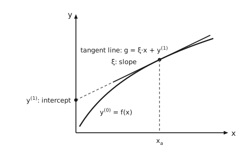
A plot with y on the vertical axis and x on the horizontal axis. A concave rising curve, steep at the left and flattening to the right, is labelled y superscript zero equals f of x. A straight tangent line lies above it and touches it at a dot above the position x sub a, joined by a dashed vertical guide. The tangent, of slope xi, is labelled g equals xi times x plus y superscript one, and is continued as a dashed line to the left to meet the vertical axis above the origin at the positive intercept y superscript one.

Figure 1 The Legendre transform as a tangent-line construction. The vertical axis is \(y\) and the horizontal axis is \(x\). A concave curve, rising steeply at the left and flattening towards the right, is the basis function \(y^{\left(0\right)} = f\left(x\right)\), labelled just below and to the right of the curve near its left end. A straight line touches it at a single point, marked with a dot, above the position \(x_{\mathrm{a}}\) on the horizontal axis. A dashed vertical guide joins the two. Because the curve bends downward, the straight line lies above it everywhere except at that point. The line is the tangent \(g = ξ \cdot x + y^{\left(1\right)}\). Its slope \(ξ\) is labelled just above it, to the left of the point of contact, and its equation is written above that, towards the point of contact. Continued as a dashed line to the left, the tangent meets the vertical axis above the origin at a second dot, which is the intercept \(y^{\left(1\right)}\), labelled to the left of the axis. The intercept is therefore positive.

Worked example: the exponential function

\[y^{\left(0\right)}\left(x\right) = f\left(x\right) = e^{x}\]
\[\implies ξ = \frac{\mathrm{d}y^{\left(0\right)}}{\mathrm{d}x} = e^{x} \implies x = \ln ξ\]
\[y^{\left(1\right)} = y^{\left(0\right)}\left(x\right) - x \cdot e^{x} = e^{x} - x \cdot e^{x} = ξ - ξ \ln ξ\]

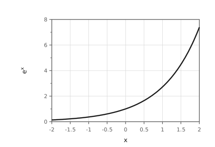
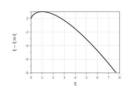
See Figure 2 and Figure 3.

A plot of e to the x against x, with x from minus 2 to 2 and the vertical axis from 0 to 8, labelled every 2 units with minor ticks at every unit. The curve is near zero at the left, passes through 1 at x equals 0, and rises steeply to about 7.4 at x equals 2.

Figure 2 The basis function \(e^{x}\). A plot of \(e^{x}\) against \(x\), with \(x\) running from −2 to 2 and the vertical axis from 0 to 8, labelled every 2 units with an unlabelled minor tick at every unit between. The curve is close to zero at the left of the range, passes through 1 at \(x = 0\), and rises steeply to about 7.4 at \(x = 2\).

A plot of xi minus xi times the natural log of xi, against xi from 0 to 8, with the vertical axis from minus 8 to 1, labelled every 2 units with minor ticks at every unit. The curve starts at zero, peaks at 1 when xi equals 1, crosses zero again near xi equals e, and then falls to about minus 7.6 at xi equals 7.5.

Figure 3 Its Legendre transform. A plot of \(ξ - ξ \ln ξ\) against \(ξ\), with \(ξ\) running from 0 to 8 and the vertical axis from −8 to 1, labelled every 2 units from −8 to 0 with an unlabelled minor tick at every unit between and at 1. The curve starts at zero, rises to a maximum of 1 at \(ξ = 1\), crosses zero again near \(ξ = e\), and then falls away, reaching about −7.6 at \(ξ = 7.5\).

Classical mechanics, with a different sign convention

\[y^{\left(1\right)}\left(ξ\right) = x \cdot ξ - y^{\left(0\right)}\left(x\right)\]

Lagrangian \(\mathcal{L}\), where \(\dot{q}\) is the velocity:

\[\mathcal{L} = \tfrac{1}{2} m \dot{q}^{2} - U\left(q\right) = \mathcal{L}\left(q, \dot{q}\right)\]
\[ξ = \frac{\partial \mathcal{L}}{\partial \dot{q}} = m \dot{q} \equiv p, \text{ the momentum}\]

Hamiltonian \(\mathcal{H}\):

\[\mathcal{H} = \dot{q} \cdot \frac{\partial \mathcal{L}}{\partial \dot{q}} - \mathcal{L} = \frac{p^{2}}{m} - \tfrac{1}{2} m \cdot \left(\frac{p}{m}\right)^{2} + U\]
\[= \frac{p^{2}}{2m} + U\left(q\right) = \mathcal{H}\left(p, q\right)\]

Two variables

In two dimensions there will be two variables:

\[y^{\left(0\right)} = f\left(x_{1}, x_{2}\right)\]
\[ξ_{1} = \left(\frac{\partial f}{\partial x_{1}}\right)_{x_{2}} \text{ and } ξ_{2} = \left(\frac{\partial f}{\partial x_{2}}\right)_{x_{1}}\]

First Legendre transform:

\[y^{\left(1\right)} = f\left(x_{1}, x_{2}\right) - ξ_{1} \cdot x_{1} = y^{\left(1\right)}\left(ξ_{1}, x_{2}\right)\]
\[\text{or } y^{\left(1\right)} = f\left(x_{1}, x_{2}\right) - ξ_{2} \cdot x_{2} = y^{\left(1\right)}\left(x_{1}, ξ_{2}\right)\]

Second Legendre transform:

\[y^{\left(2\right)} = f\left(x_{1}, x_{2}\right) - ξ_{1} \cdot x_{1} - ξ_{2} \cdot x_{2} = y^{\left(2\right)}\left(ξ_{1}, ξ_{2}\right)\]

Many variables

\[y^{\left(0\right)} = f\left(x_{1}, x_{2}, \dots, x_{m}\right) \text{ with } ξ_{i} = \left(\frac{\partial f}{\partial x_{i}}\right)_{x_{j \ne i}}\]

The \(k\)-th Legendre transform:

\[y^{\left(k\right)} = y^{\left(0\right)} - \sum_{i=1}^{k} ξ_{i} \cdot x_{i} = y^{\left(k\right)}\left(ξ_{1}, ξ_{2}, \dots, ξ_{k}, x_{k+1}, \dots, x_{m}\right)\]

Differentiating,

\[\mathrm{d}y^{\left(0\right)} = \sum_{i=1}^{m} ξ_{i} \cdot \mathrm{d}x_{i}\]

This shows \(y^{\left(k\right)}\) is a function of \(ξ_{1}, ξ_{2}, \dots, ξ_{k}, x_{k+1}, \dots, x_{m}\).

Application to thermodynamics

Take the basis function to be the internal energy, whose \(N + 2\) arguments are numbered \(x_{1}\) through \(x_{N+2}\):

Table 1 The variables of the energy representation and their conjugates. For each index \(i\), the variable \(x_{i}\) and its conjugate \(ξ_{i} = \left(\partial U / \partial x_{i}\right)\).

\(i\)

\(x_{i}\)

\(ξ_{i}\)

1

\(S\)

\(T\)

2

\(V\)

\(- P\)

3

\(n_{1}\)

\(μ_{1}\)

\(\vdots\)

\(\vdots\)

\(\vdots\)

\(N + 2\)

\(n_{N}\)

\(μ_{N}\)

Transforming on row 2 leaves \(S, - P\) and the mole numbers, which are the independent variables of the enthalpy:

\[y^{\left(1\right)} = U - V \cdot \left(- P\right) \equiv H\]

Transforming on row 1 leaves \(T, V\) and the mole numbers, which are those of the Helmholtz energy:

\[y^{\left(1\right)} = U - S \cdot T \equiv A\]

Transforming on the first two rows leaves \(T, - P\) and the mole numbers, which are the independent variables of the Gibbs energy:

\[y^{\left(2\right)} = U + V \cdot P - S \cdot T \equiv G\]

The corresponding differential relations are

\[\mathrm{d}H = T \mathrm{d}S - P \mathrm{d}V + \sum μ_{i} \mathrm{d}n_{i} - \mathrm{d}\left[\left(- P\right) \cdot V\right]\]
\[= T \mathrm{d}S + V \mathrm{d}P + \sum μ_{i} \mathrm{d}n_{i}\]
\[\mathrm{d}A = - S \mathrm{d}T - P \mathrm{d}V + \sum μ_{i} \mathrm{d}n_{i}\]
\[\mathrm{d}G = - S \mathrm{d}T + V \mathrm{d}P + \sum μ_{i} \mathrm{d}n_{i}\]

Total Legendre transform and the Gibbs-Duhem equation

\[y^{\left(N+2\right)} = U - TS + PV - \sum μ_{i} \cdot n_{i}\]

Applying Euler’s theorem for \(U = U\left(S, V, n_{i}\right)\) we get

\[U = TS - PV + \sum μ_{i} \cdot n_{i}\]

Therefore \(y^{\left(N+2\right)} = 0\), so \(\mathrm{d}y^{\left(N+2\right)} = 0\), or

\[- S \mathrm{d}T + V \mathrm{d}P - \sum n_{i} \mathrm{d}μ_{i} = 0 \qquad \text{(Gibbs-Duhem)}\]

Euler’s theorem for homogeneous functions

Consider \(y = f\left(x\right)\). The two statements

(1)\[f\left(kx\right) = k^{h} \cdot f\left(x\right)\]
(2)\[x \cdot f'\left(x\right) = h \cdot f\left(x\right)\]

are equivalent: each implies the other. We call \(f\left(x\right)\) a homogeneous function of order \(h\).

Proof:

  • First direction, that Equation (2) implies Equation (1). From Equation (2), \(kx \cdot f' \left(kx\right) = h \cdot f\left(kx\right)\). Let \(g\left(k\right) = f\left(kx\right)\). Then

\[\frac{\mathrm{d}g}{\mathrm{d}k} = g' \left(k\right) = x \cdot f' \left(kx\right) = \frac{h}{k} f\left(kx\right) = \frac{h}{k} g\left(k\right)\]
\[\frac{\mathrm{d}g}{g} = \frac{h}{k} \mathrm{d}k \implies g\left(k\right) = g\left(1\right) \cdot k^{h}\]

This is Equation (1): \(f\left(kx\right) = f\left(x\right) \cdot k^{h}\).

\[\frac{\partial \left[f\left(kx\right)\right]}{\partial k} = \frac{\partial \left[k^{h} \cdot f\left(x\right)\right]}{\partial k}\]

The two sides give

\[\text{LHS} = x \cdot f'\left(kx\right)\]
\[\text{RHS} = h \cdot k^{h-1} \cdot f\left(x\right)\]

so that \(x \cdot f'\left(kx\right) = h \cdot k^{h-1} \cdot f\left(x\right)\). Let \(k = 1\): then \(x \cdot f' \left(x\right) = h \cdot f\left(x\right)\), which is Equation (2).

One can also show

\[f\left(a, b, kx, ky\right) = k^{h} f\left(a, b, x, y\right)\]
\[⟺ x \cdot f'_{x} + y \cdot f'_{y} = h \cdot f\left(a, b, x, y\right)\]

The internal energy \(U = U\left(S, V, n_{1}, n_{2}, \dots, n_{N}\right)\) is a homogeneous function of order 1, that is,

\[U\left(kS, kV, kn_{1}, kn_{2}, \dots, kn_{N}\right) = k^{1} \cdot U\left(S, V, n_{1}, n_{2}, \dots, n_{N}\right)\]

Therefore

\[S \cdot \left(\frac{\partial U}{\partial S}\right) + V \cdot \left(\frac{\partial U}{\partial V}\right) + \sum n_{i} \frac{\partial U}{\partial n_{i}} = 1 \cdot U\]

or

\[S \cdot T + V \cdot \left(- P\right) + \sum n_{i} \cdot μ_{i} = U\]

so that

\[U - TS + PV - \sum μ_{i} n_{i} = 0\]

Likewise, for the Gibbs energy,

\[G\left(T, P, kn_{1}, kn_{2}, \dots, kn_{N}\right) = k G\left(T, P, n_{1}, n_{2}, \dots, n_{N}\right)\]
\[\sum n_{i} \cdot \frac{\partial G}{\partial n_{i}} = 1 \cdot G \implies G = \sum n_{i} \cdot \tilde{G}_{i} = \sum n_{i} \cdot μ_{i}\]

Extensive versus intensive properties

The extensive properties are \(U, S, V, N\) and \(H, A, G\). The intensive variables come in two kinds:

  1. field variables: \(T, P, μ_{i}\);

  2. density variables: \(\tilde{V} = \frac{V}{N}\) and \(\tilde{U} = \frac{U}{N}\).

\[\left(\frac{\partial U}{\partial N}\right)_{S,\, V} = μ = \left[\frac{\partial \left(N \tilde{U}\right)}{\partial N}\right]_{S,\, V} = \tilde{U} + N\left(\frac{\partial \tilde{U}}{\partial N}\right)_{S,\, V}\]

Both \(\left(\frac{\partial U}{\partial N}\right)_{S,\, V}\) and \(\left(\frac{\partial \tilde{U}}{\partial N}\right)_{S,\, V}\) are non-zero, whereas

\[\left(\frac{\partial \tilde{U}}{\partial N}\right)_{\tilde{S},\, \tilde{V}} = 0\]

which follows from \(\tilde{U}\left(\tilde{S}, \tilde{V}, kN\right) = k^{0} \tilde{U}\left(\tilde{S}, \tilde{V}, N\right)\) and

\[\left(\frac{\partial \tilde{U}}{\partial N}\right) \cdot N = 0 \cdot \tilde{U} = 0\]

Hence

Maxwell relations

For \(f\left(x_{1}, x_{2}\right)\):

\[\frac{\partial}{\partial x_{2}}\left(\frac{\partial f}{\partial x_{1}}\right) = \frac{\partial}{\partial x_{1}}\left(\frac{\partial f}{\partial x_{2}}\right), \text{ or } f_{x_{1},x_{2}} = f_{x_{2},x_{1}}\]
Table 2 The Maxwell relations. Each fundamental relation and the Maxwell relation that follows from it.

Fundamental relation

Maxwell relation

\(\mathrm{d}U = T\mathrm{d}S - P\mathrm{d}V\)

\(\left(\frac{\partial T}{\partial V}\right)_{S} = - \left(\frac{\partial P}{\partial S}\right)_{V}\)

\(\mathrm{d}H = T\mathrm{d}S + V\mathrm{d}P\)

\(\left(\frac{\partial T}{\partial P}\right)_{S} = \left(\frac{\partial V}{\partial S}\right)_{P}\)

\(\mathrm{d}A = - S\mathrm{d}T - P\mathrm{d}V\)

\(\left(\frac{\partial S}{\partial V}\right)_{T} = \left(\frac{\partial P}{\partial T}\right)_{V}\)

\(\mathrm{d}G = - S\mathrm{d}T + V\mathrm{d}P\)

\(- \left(\frac{\partial S}{\partial P}\right)_{T} = \left(\frac{\partial V}{\partial T}\right)_{P}\)

The last two relations are particularly useful (e.g., used repeatedly in the examples below) because the awkard derivatives on the left-hand side involving entropy are converted to derivatives based on the \(pVT\) relationship.

Tools for transforming derivatives

  1. The Maxwell relations above.

  2. Chain rule:

    \[\left(\frac{\partial F}{\partial y}\right)_{x} = \left(\frac{\partial F}{\partial φ}\right)_{x} \cdot \left(\frac{\partial φ}{\partial y}\right)_{x}\]
  3. Cyclic rule, or triple product:

    \[\left(\frac{\partial y}{\partial x}\right)_{z} \cdot \left(\frac{\partial x}{\partial z}\right)_{y} \cdot \left(\frac{\partial z}{\partial y}\right)_{x} = - 1\]
  4. Derivative inversion:

    \[\left(\frac{\partial F}{\partial y}\right)_{x} = \left(\frac{\partial y}{\partial F}\right)_{x}^{- 1}\]
  5. Euler integration:

    \[U = U\left(S, V, N\right) = S \cdot \frac{\partial U}{\partial S} + V \cdot \frac{\partial U}{\partial V} + N \cdot \frac{\partial U}{\partial N}\]
    \[G = G\left(T, P, N\right) = N \cdot \frac{\partial G}{\partial N} = N \cdot μ\]
  6. Manipulate the total derivative for \(F\left(x, y\right)\):

    \[\mathrm{d}F = \left(\frac{\partial F}{\partial x}\right)_{y} \mathrm{d}x + \left(\frac{\partial F}{\partial y}\right)_{x} \mathrm{d}y\]

Examples

Example: enthalpy as a function of temperature and pressure, \(\tilde{H} = f\left(T, P\right)\)

The second coefficient is the derivative that has to be found. The fully specified differential form can be used to calculate \(\Delta H\) (Figure 4).
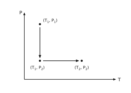
A pressure-temperature diagram with three marked states. An arrow runs straight down from the state at T sub 1 and P sub 1 to the state at T sub 1 and P sub 2, then straight right to the state at T sub 2 and P sub 2.

Figure 4 The two-step path used for the enthalpy example. The vertical axis is \(P\) and the horizontal axis is \(T\). Three states are marked with dots. From \(\left(T_{1}, P_{1}\right)\) at the upper left, an arrow points straight down to \(\left(T_{1}, P_{2}\right)\), a change of pressure at constant temperature. From there an arrow points straight right to \(\left(T_{2}, P_{2}\right)\), a change of temperature at constant pressure.

From \(\mathrm{d}H = T \mathrm{d}S + V \mathrm{d}P\),

\[\left(\frac{\partial \tilde{H}}{\partial P}\right)_{T} = T \left(\frac{\partial \tilde{S}}{\partial P}\right)_{T} + \tilde{V} = T\left[- \left(\frac{\partial \tilde{V}}{\partial T}\right)_{P}\right] + \tilde{V}\]

using the Maxwell relation based on the Gibbs energy expression. Hence

\[\mathrm{d}\tilde{H} = \tilde{C}_{P} \mathrm{d}T + \left[\tilde{V} - T\left(\frac{\partial \tilde{V}}{\partial T}\right)_{P}\right] \mathrm{d}P\]
  • For ideal gases, \(P\tilde{V} = RT\), so \(\tilde{V} = \frac{RT}{P}\) and \(\left(\frac{\partial \tilde{V}}{\partial T}\right)_{P} = \frac{R}{P}\). Then

\[\tilde{V} - T\left(\frac{\partial \tilde{V}}{\partial T}\right)_{P} = \tilde{V} - \frac{RT}{P} = 0\]

leaving

\[\mathrm{d}\tilde{H} = \tilde{C}_{P} \mathrm{d}T\]
  • For solids and liquids, define the isobaric thermal expansion coefficient

\[β = \frac{1}{\tilde{V}} \left(\frac{\partial \tilde{V}}{\partial T}\right)_{P}\]

so that

\[\mathrm{d}\tilde{H} = \tilde{C}_{P} \mathrm{d}T + \left(\tilde{V} - βT\tilde{V}\right) \mathrm{d}P = \tilde{C}_{P} \mathrm{d}T + \left(1 - βT\right) \tilde{V} \mathrm{d}P\]

Example: entropy as a function of temperature and pressure, \(\tilde{S} = f\left(T, P\right)\)

The fundamental equation \(\mathrm{d}\tilde{S} = \frac{\mathrm{d}\tilde{U}}{T} + \frac{P}{T} \mathrm{d}\tilde{V}\) has different independent variables. We need

\[\mathrm{d}\tilde{S} = \left(\frac{\partial \tilde{S}}{\partial T}\right)_{P} \mathrm{d}T + \left(\frac{\partial \tilde{S}}{\partial P}\right)_{T} \mathrm{d}P\]

with \(\left(\frac{\partial \tilde{S}}{\partial P}\right)_{T} = - \left(\frac{\partial \tilde{V}}{\partial T}\right)_{P}\). At constant pressure the second term of the enthalpy relation drops out,

and

\[\left(\frac{\partial \tilde{H}}{\partial T}\right)_{P} = T\left(\frac{\partial \tilde{S}}{\partial T}\right)_{P} = \tilde{C}_{P}\]

so that

\[\mathrm{d}\tilde{S} = \frac{\tilde{C}_{P}}{T} \mathrm{d}T - \left(\frac{\partial \tilde{V}}{\partial T}\right)_{P} \mathrm{d}P\]

One can also express \(\left(\frac{\partial \tilde{V}}{\partial T}\right)_{P} = β\tilde{V}\).

  • For ideal gases, \(P\tilde{V} = RT\) gives \(\tilde{V} = \frac{RT}{P}\), so

\[\mathrm{d}\tilde{S} = \frac{\tilde{C}_{P}}{T} \mathrm{d}T - \frac{R}{P} \mathrm{d}P\]
\[ΔS = S_{2} - S_{1} = \tilde{C}_{P} \ln \frac{T_{2}}{T_{1}} - R \ln \frac{P_{2}}{P_{1}}\]

Example: internal energy as a function of temperature and molar volume, \(\tilde{U} = f\left(T, \tilde{V}\right)\)

From \(\mathrm{d}\tilde{U} = T \mathrm{d}\tilde{S} - P \mathrm{d}\tilde{V}\), and the Maxwell relation based on the Helmholtz energy expression,

\[\left(\frac{\partial \tilde{U}}{\partial \tilde{V}}\right)_{T} = T\left(\frac{\partial \tilde{S}}{\partial \tilde{V}}\right)_{T} - P = T\left(\frac{\partial P}{\partial T}\right)_{\tilde{V}} - P\]

so that

\[\mathrm{d}\tilde{U} = \tilde{C}_{V} \mathrm{d}T + \left[T\left(\frac{\partial P}{\partial T}\right)_{\tilde{V}} - P\right] \mathrm{d}\tilde{V}\]
  • For ideal gases, \(P\tilde{V} = RT\) and \(\frac{\partial P}{\partial T} = \frac{R}{\tilde{V}}\), so

\[T\left(\frac{\partial P}{\partial T}\right)_{\tilde{V}} - P = \frac{RT}{\tilde{V}} - P = 0\]

leaving

\[\mathrm{d}\tilde{U} = \tilde{C}_{V} \mathrm{d}T\]
  • For a van der Waals fluid, with \(a\) and \(b\) constant,

\[P = \frac{RT}{\tilde{V} - b} - \frac{a}{\tilde{V}^{2}}\]
\[\left(\frac{\partial P}{\partial T}\right)_{\tilde{V}} = \frac{R}{\tilde{V} - b}\]

so

\[\mathrm{d}\tilde{U} = \tilde{C}_{V} \mathrm{d}T + \frac{a}{\tilde{V}^{2}} \mathrm{d}\tilde{V}\]
\[Δ\tilde{U} = \tilde{U}_{2} - \tilde{U}_{1} = \tilde{C}_{V}\left(T_{2} - T_{1}\right) - a\left(\frac{1}{\tilde{V}_{2}} - \frac{1}{\tilde{V}_{1}}\right)\]

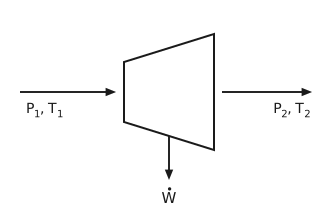
Example: working fluid in a turbine

A turbine drawn as a quadrilateral, narrow at the inlet and wider at the outlet. An arrow enters from the left labelled beneath P sub 1 and T sub 1, an arrow leaves to the right labelled beneath P sub 2 and T sub 2, and an arrow points downward from the bottom carrying the shaft power W dot.

Figure 5 Working fluid in a turbine. The turbine is drawn as a quadrilateral, narrow at the inlet on the left and wider at the outlet on the right. An arrow enters from the left carrying the feed, labelled \(P_{1}, T_{1}\) beneath it near its tail. An arrow leaves to the right at the same height, carrying the discharge, labelled \(P_{2}, T_{2}\) beneath it near its head, so the two labels are level. A third arrow points downward out of the bottom of the body, carrying the shaft power \(\dot{W}\).

Figure 5: Given \(ΔP\), the larger the \(ΔT\), the better. The figure of merit is therefore

\[α_{S} = \left(\frac{\partial T}{\partial P}\right)_{\tilde{S}}\]

The Maxwell relation based on the enthalpy expression gives \(\left(\frac{\partial T}{\partial P}\right)_{\tilde{S}} = \left(\frac{\partial \tilde{V}}{\partial \tilde{S}}\right)_{P}\), which does not seem to be very useful.

Apply the cyclic rule instead and use derivative inversion and another Maxwell relation based on the Gibbs energy expression:

\[α_{S} = \left(\frac{\partial T}{\partial P}\right)_{\tilde{S}} = - \left(\frac{\partial \tilde{S}}{\partial P}\right)_{T} \cdot \left(\frac{\partial T}{\partial \tilde{S}}\right)_{P} = \left(\frac{\partial \tilde{V}}{\partial T}\right)_{P} \cdot \left(\frac{\partial T}{\partial \tilde{S}}\right)_{P}\]

At constant pressure the last term of the enthalpy relation drops out again,

so that \(\tilde{C}_{P} = T\left(\frac{\partial \tilde{S}}{\partial T}\right)_{P}\), which is the reciprocal of the last factor above. Therefore

\[α_{S} = \frac{T}{\tilde{C}_{P}} \left(\frac{\partial \tilde{V}}{\partial T}\right)_{P}\]
  • For ideal gases,

\[α_{S} = \frac{T}{\tilde{C}_{P}} \cdot \frac{\partial}{\partial T}\left(\frac{RT}{P}\right)_{P} = \frac{RT}{\tilde{C}_{P} \cdot P} = \frac{\tilde{V}}{\tilde{C}_{P}}\]

Example: the Joule-Thomson coefficient

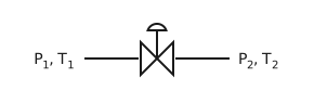
Cooling by expansion (Figure 6).

A horizontal pipe interrupted at its midpoint by a valve drawn as two triangles meeting point to point, with a domed knob on a stem above it. The upstream side is labelled P sub 1 and T sub 1 and the downstream side P sub 2 and T sub 2.

Figure 6 The throttle of the Joule-Thomson example. A horizontal pipe is interrupted at its midpoint by a valve, drawn as two triangles meeting point to point. A knob, the top third of a circle, sits above the valve on a vertical stem that comes down to the point where the triangles meet. The upstream side, to the left, is at \(P_{1}, T_{1}\) and the downstream side, to the right, is at \(P_{2}, T_{2}\).

Previously we showed \(ΔH = 0\), an isenthalpic expansion. Given \(P_{1}\) and \(P_{2}\), how much does it cool?

\[α_{H} = \left(\frac{\partial T}{\partial P}\right)_{\tilde{H}}\]

Apply the cyclic rule:

From \(\mathrm{d}\tilde{H} = T \mathrm{d}\tilde{S} + \tilde{V} \mathrm{d}P\),

\[\left(\frac{\partial \tilde{H}}{\partial P}\right)_{T} = T \left(\frac{\partial \tilde{S}}{\partial P}\right)_{T} + \tilde{V} = T\left[- \left(\frac{\partial \tilde{V}}{\partial T}\right)_{P}\right] + \tilde{V}\]

again using the Maxwell relation based on the Gibbs energy expression. Hence

\[\tilde{α}_{H} = - \frac{1}{\tilde{C}_{P}} \left[\tilde{V} - T\left(\frac{\partial \tilde{V}}{\partial T}\right)_{P}\right]\]
  • For ideal gases, \(P\tilde{V} = RT\) and \(\frac{\partial \tilde{V}}{\partial T} = \frac{R}{P}\), so

\[\tilde{α}_{H} = 0\]

Example: is the difference of the heat capacities (\(\tilde{C}_{P} - \tilde{C}_{V}\)) always \(R\)?

\[\mathrm{d}\tilde{H} = T \mathrm{d}\tilde{S} + \tilde{V} \mathrm{d}P \implies \tilde{C}_{P} = \left(\frac{\partial \tilde{H}}{\partial T}\right)_{P} = T\left(\frac{\partial \tilde{S}}{\partial T}\right)_{P}\]
\[\mathrm{d}\tilde{U} = T \mathrm{d}\tilde{S} - P \mathrm{d}\tilde{V} \implies \tilde{C}_{V} = \left(\frac{\partial \tilde{U}}{\partial T}\right)_{\tilde{V}} = T \left(\frac{\partial \tilde{S}}{\partial T}\right)_{\tilde{V}}\]
\[\therefore \tilde{C}_{P} - \tilde{C}_{V} = T \left[\left(\frac{\partial \tilde{S}}{\partial T}\right)_{P} - \left(\frac{\partial \tilde{S}}{\partial T}\right)_{\tilde{V}}\right]\]

Expanding the entropy in \(T\) and \(\tilde{V}\),

\[\mathrm{d}\tilde{S} = \left(\frac{\partial \tilde{S}}{\partial T}\right)_{\tilde{V}} \mathrm{d}T + \left(\frac{\partial \tilde{S}}{\partial \tilde{V}}\right)_{T} \mathrm{d}\tilde{V}\]
\[\implies \left(\frac{\partial \tilde{S}}{\partial T}\right)_{P} = \left(\frac{\partial \tilde{S}}{\partial T}\right)_{\tilde{V}} + \left(\frac{\partial \tilde{S}}{\partial \tilde{V}}\right)_{T} \left(\frac{\partial \tilde{V}}{\partial T}\right)_{P}\]

so that, for any material,

\[\tilde{C}_{P} - \tilde{C}_{V} = T \left(\frac{\partial \tilde{S}}{\partial \tilde{V}}\right)_{T} \cdot \left(\frac{\partial \tilde{V}}{\partial T}\right)_{P} = T \left(\frac{\partial P}{\partial T}\right)_{\tilde{V}} \cdot \left(\frac{\partial \tilde{V}}{\partial T}\right)_{P}\]
  • For ideal gases, \(\tilde{C}_{P} - \tilde{C}_{V} = R\).

  • For solids and liquids, we often use the isobaric thermal expansion coefficient and the isothermal compressibility:

\[β = \frac{1}{\tilde{V}} \left(\frac{\partial \tilde{V}}{\partial T}\right)_{P}\]
\[κ = - \frac{1}{\tilde{V}} \left(\frac{\partial \tilde{V}}{\partial P}\right)_{T}\]

If incompressible, \(β = κ = 0\) and

\[\tilde{C}_{P} - \tilde{C}_{V} = 0\]

Example: constructing the molar entropy of a monatomic gas

Construct \(\tilde{S}\left(\tilde{U}, \tilde{V}\right)\) for a monatomic gas using \(P\tilde{V} = RT\) and \(\tilde{C}_{V} = \frac{3}{2}R\).

\[\mathrm{d}\tilde{S} = \left(\frac{\partial \tilde{S}}{\partial \tilde{U}}\right)_{\tilde{V}} \mathrm{d}\tilde{U} + \left(\frac{\partial \tilde{S}}{\partial \tilde{V}}\right)_{\tilde{U}} \mathrm{d}\tilde{V}\]
\[\mathrm{d}\tilde{S} = \frac{\mathrm{d}\tilde{U}}{T} + \frac{P \mathrm{d}\tilde{V}}{T}\]

the second line following from \(\mathrm{d}\tilde{U} = T \mathrm{d}\tilde{S} - P \mathrm{d}\tilde{V}\). To integrate, we need to express \(T\) and \(\frac{P}{T}\) as a function of \(\tilde{U}\) and \(\tilde{V}\):

\[\frac{P}{T} = \frac{R}{\tilde{V}}\]
\[\left(\frac{\mathrm{d}\tilde{U}}{\mathrm{d}T}\right)_{\tilde{V}} = \tilde{C}_{V} = \frac{3}{2}R \implies \tilde{U} - \tilde{U}_{0} = \frac{3}{2} R \left(T - T_{0}\right)\]

Then

\[\mathrm{d}\tilde{S} = \frac{3}{2}R \cdot \frac{\mathrm{d}\tilde{U}}{\tilde{U}} + R \cdot \frac{\mathrm{d}\tilde{V}}{\tilde{V}}\]
\[\tilde{S} = \tilde{S}_{0} + \frac{3}{2}R \ln \frac{\tilde{U}}{\tilde{U}_{0}} + R \ln \frac{\tilde{V}}{\tilde{V}_{0}} = \tilde{S}_{0} + R \ln \left[\left(\frac{\tilde{U}}{\tilde{U}_{0}}\right)^{3/2} \cdot \left(\frac{\tilde{V}}{\tilde{V}_{0}}\right)\right]\]

or

\[S = S_{0} + nR \ln \left[\left(\frac{U}{U_{0}}\right)^{3/2} \cdot \left(\frac{V}{V_{0}}\right)\right]\]

Example: constructing the molar Gibbs energy of an arbitrary material

Construct \(\tilde{G}\left(T, P\right)\) for an arbitrary material using \(β\) and \(κ\), and \(\tilde{C}_{P}\).

First note that, by Euler integration,

\[G\left(T, P, n\right) = n \cdot \left(\frac{\partial G}{\partial n}\right)_{P,\, T} = n \cdot μ\]

so that \(\frac{G}{n} = μ = \tilde{G}\), and

\[\mathrm{d}μ = \mathrm{d}\tilde{G} = \left(\frac{\partial \tilde{G}}{\partial T}\right)_{P} \mathrm{d}T + \left(\frac{\partial \tilde{G}}{\partial P}\right)_{T} \mathrm{d}P = - \tilde{S} \mathrm{d}T + \tilde{V} \mathrm{d}P\]

To integrate, we need to express \(\tilde{S}\) and \(\tilde{V}\) as a function of \(T\) and \(P\). Previously,

\[\mathrm{d}\tilde{S} = \frac{\tilde{C}_{P}}{T} \mathrm{d}T - \left(\frac{\partial \tilde{V}}{\partial T}\right)_{P} \mathrm{d}P = \frac{\tilde{C}_{P}}{T} \mathrm{d}T - β\tilde{V} \mathrm{d}P\]
\[\implies \tilde{S} = \tilde{S}_{0} + \int_{T_{0}}^{T} \frac{\tilde{C}_{P}}{T} \mathrm{d}T - \int_{P_{0}}^{P} β\tilde{V} \mathrm{d}P\]

and likewise

\[\mathrm{d}\tilde{V} = \left(\frac{\partial \tilde{V}}{\partial T}\right)_{P} \mathrm{d}T + \left(\frac{\partial \tilde{V}}{\partial P}\right)_{T} \mathrm{d}P = β\tilde{V} \mathrm{d}T - κ\tilde{V} \mathrm{d}P\]
\[\implies \tilde{V} = \tilde{V}_{0} + \int_{T_{0}}^{T} β\tilde{V} \mathrm{d}T - \int_{P_{0}}^{P} κ\tilde{V} \mathrm{d}P\]

Now we integrate \(μ\), or \(\tilde{G}\), along the path depicted in Figure 7.
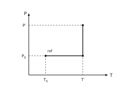
A pressure-temperature diagram. Dashed guides mark P sub 0 and P prime on the vertical axis and T sub 0 and T prime on the horizontal axis. A heavy path runs from the reference state at T sub 0 and P sub 0, marked ref, horizontally right at constant pressure to T prime, then vertically up at constant temperature to P prime.

Figure 7 The integration path from the reference state. The vertical axis is \(P\) and the horizontal axis is \(T\). Dashed guide lines mark \(P_{0}\) and \(P'\) on the vertical axis and \(T_{0}\) and \(T'\) on the horizontal axis, closing a rectangle between the reference corner and the target corner. Three states are marked with dots. The heavy path runs from the reference state at \(\left(T_{0}, P_{0}\right)\), labelled “ref”, horizontally right along the constant pressure \(P_{0}\) to \(\left(T', P_{0}\right)\), and then vertically up along the constant temperature \(T'\) to \(\left(T', P' \right)\). The first leg therefore contributes the temperature integral at the reference pressure, and the second the pressure integral at the final temperature.

The pressure integral in the first bracket is zero because that leg is walked at \(P = P_{0}\). Integrating gives

which is a general expression valid for any material.

  • For an ideal gas,

\[β = \frac{1}{\tilde{V}} \left(\frac{\partial \tilde{V}}{\partial T}\right)_{P} = \frac{1}{\tilde{V}}\,\frac{\partial}{\partial T}\left(\frac{RT}{P}\right) = \frac{R}{P\tilde{V}} = \frac{1}{T}\]
\[κ = - \frac{1}{\tilde{V}} \left(\frac{\partial \tilde{V}}{\partial P}\right)_{T} = - \frac{1}{\tilde{V}}\,\frac{\partial}{\partial P}\left(\frac{RT}{P}\right) = \frac{RT}{P^{2}\tilde{V}} = \frac{1}{P}\]

so the two inner integrals are

\[\int_{T_{0}}^{T'} β\tilde{V} \mathrm{d}T = \int_{T_{0}}^{T'} \frac{\tilde{V}}{T} \mathrm{d}T = \int_{T_{0}}^{T'} \frac{R}{P_{0}} \mathrm{d}T = \frac{R}{P_{0}}\left(T' - T_{0}\right)\]
\[\int_{P_{0}}^{P} κ\tilde{V} \mathrm{d}P = \int_{P_{0}}^{P} \frac{\tilde{V}}{P} \mathrm{d}P = \int_{P_{0}}^{P} \frac{RT'}{P^{2}} \mathrm{d}P = - RT' \left(\frac{1}{P} - \frac{1}{P_{0}}\right)\]

Therefore

Hence, for an ideal gas,

We can therefore write

\[μ = μ^{\circ}\left(T\right) + RT \ln \frac{P}{P^{\circ}}\]