Stability

ChE 621 — Thermodynamics.

Classification of equilibrium states

Equilibrium states are classified based on the local curvature around the equilibrium state.
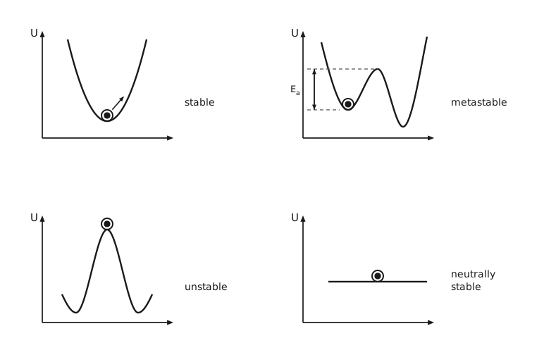
Four small plots of U against a generalized displacement, each with a marble on the curve. Stable: a single well with the marble at the bottom and an arrow pointing from the marble up the inside of the wall. Metastable: a shallow well, a barrier of height E sub a measured from the bottom of the shallow well, then a deeper well, with the marble in the shallow well. Unstable: the marble balanced on a summit, with a well on either side. Neutrally stable: a horizontal line with the marble resting on it.

Figure 1 The four classes of equilibrium state. Four small plots of \(U\) against a generalized displacement, each with a marble resting on the curve. Top left, stable: a single well, with the marble at the bottom and a short arrow pointing from the marble up the inside of the right-hand wall of the well. Top right, metastable: a shallow well on the left, then a barrier, then a deeper well on the right; the marble sits in the shallow well, and a vertical double-headed arrow between two dashed guide lines measures the barrier height \(E_{\mathrm{a}}\) from the bottom of the shallow well up to the top of the barrier. Bottom left, unstable: the marble balances on the summit of a hill, with a well on either side of it. Bottom right, neutrally stable: the curve is a horizontal line and the marble rests anywhere on it.

Stability criteria

Consider the stability of phase \(α\) with respect to the formation of another phase, \(β\), as shown in Figure 2.
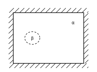
A rectangular enclosure with hatching along all four outer edges. The interior is labelled alpha, and a small dashed oval near the lower left is labelled beta.

Figure 2 A nucleus of phase \(β\) inside phase \(α\). A rectangular enclosure with hatching along all four outer edges, marking rigid walls. The interior is phase \(α\), labelled at its upper right. A small dashed oval near the lower left is a nucleus of the new phase \(β\), labelled inside the oval. The dashed outline marks it as an incipient region rather than a physical wall.

Expansion around equilibrium of the total derivative of

\[U\left(S, \vec{x}\right) = U\left(S, V, n_{1}, n_{2}, \dots, n_{N}\right) = U\left(z_{i}\right), \quad \text{where } i = 1, 2, \ldots, N+2\]

Then

\[\mathrm{d}U = δU + \frac{1}{2!} δ^{2}U + \frac{1}{3!} δ^{3}U + \dots\]

with

\[δU = \sum_{i=1}^{n+2} \left(\frac{\partial U}{\partial z_{i}}\right) δz_{i}\]
\[δ^{2}U = \sum_{i=1}^{n+2} \sum_{j=1}^{n+2} \left(\frac{\partial ^{2}U}{\partial z_{i}\cdot \partial z_{j}}\right) δz_{i} \cdot δz_{j}\]

and the displacements measured from the equilibrium value:

\[δz_{i} = z_{i} - z_{i}^{\mathrm{e}}\]

\(U\) is at a minimum at \(\vec{z}^{\mathrm{e}}\) if and only if

  • \(δU = 0\);

  • \(δ^{2}U \ge 0\), and if \(δ^{2}U = 0\), then

  • \(δ^{3}U \ge 0\), and if \(δ^{3}U = 0\), then \(δ^{4}U\), and so on, until the lowest non-vanishing term \(δ^{n}U > 0\).

The second variation for two phases

\[\begin{split}\begin{aligned} \mathrm{d}^{2}U &= \mathrm{d}^{2}U^{α} + \mathrm{d}^{2}U^{β} \\ &= U_{SS}^{α} \left(\mathrm{d}S^{α}\right)^{2} + U_{VV}^{α} \left(\mathrm{d}V^{α}\right)^{2} + U_{NN}^{α} \left(\mathrm{d}N\right)^{2} + 2U_{SV}^{α} \mathrm{d}S^{α} \mathrm{d}V^{α} \\ &\quad + 2U_{SN}^{α} \mathrm{d}S^{α} \mathrm{d}N^{α} + 2U_{VN}^{α} \mathrm{d}V^{α} \mathrm{d}N^{α} + \text{terms for } β \end{aligned}\end{split}\]

where

\[U_{SS}^{α} = \frac{\partial ^{2}U^{α}}{\partial S\cdot \partial S}, \qquad U_{SV}^{α} = \frac{\partial ^{2}U^{α}}{\partial S\cdot \partial V}, \qquad \dots\]

Because phases \(α\) and \(β\) are initially identical, two consequences follow together:

The second follows because

Therefore

\[\mathrm{d}^{2}U = \left(1 + \frac{N^{α}}{N^{β}}\right) \mathrm{d}^{2}U^{α} > 0, \text{ or } \mathrm{d}^{2}U^{α} > 0\]

Drop the superscript \(α\), so that

(1)\[\begin{split}\begin{aligned} \mathrm{d}^{2}U = {} & U_{SS}\left(\mathrm{d}S\right)^{2} + U_{VV}\left(\mathrm{d}V\right)^{2} + U_{NN}\left(\mathrm{d}N\right)^{2} \\ & + 2U_{SV}\left(\mathrm{d}S\right)\left(\mathrm{d}V\right) + 2U_{VN}\left(\mathrm{d}V\right)\left(\mathrm{d}N\right) \\ & + 2U_{SN}\left(\mathrm{d}S\right)\left(\mathrm{d}N\right) > 0 \end{aligned}\end{split}\]

The Hessian form

For \(n\)-component systems,

The second variation is the quadratic form

The matrix in the middle, \(\bar{\bar{H}}\), is the \(m \times m\) Hessian matrix of second derivatives; it is also Hermitian. In the compact form,

\[δ^{2}U = δ\vec{z}^{\mathrm{T}} \cdot \bar{\bar{H}} \cdot δ\vec{z}\]

and \(\bar{\bar{H}}\) is positive definite if and only if \(|\bar{\bar{H}}| > 0\).

Example: two variables

For \(\tilde{U} = \tilde{U}\left(\tilde{S}, \tilde{V}\right)\), the determinant of the two-by-two Hessian must be positive:

Reducing Equation (1) to a diagonal form

Back to Equation (1), one can eliminate the cross terms and get

\[\mathrm{d}^{2}U = \frac{1}{U_{SS}}\left(\mathrm{d}T\right)^{2} + \frac{1}{A_{VV}}\left(\mathrm{d}P\right)^{2} > 0\]

where

\[A_{VV} = \left(\frac{\partial ^{2}A}{\partial V^{2}}\right)_{T,\, N}\]

Stability therefore requires \(U_{SS} > 0\) and \(A_{VV} > 0\), which are

\[U_{SS} = \left(\frac{\partial T}{\partial S}\right)_{V,\, N} = \frac{T}{C_{V}} > 0 \implies C_{V} > 0 \qquad \text{(thermal)}\]
\[A_{VV} = - \left(\frac{\partial P}{\partial V}\right)_{T,\, N} > 0, \text{ or } \left(\frac{\partial P}{\partial V}\right)_{T,\, N} < 0 \qquad \text{(mechanical)}\]

Derivation

\[\mathrm{d}T = \left(\frac{\partial T}{\partial S}\right)_{V,\, N} \mathrm{d}S + \left(\frac{\partial T}{\partial V}\right)_{S,\, N} \mathrm{d}V + \left(\frac{\partial T}{\partial N}\right)_{S,\, V} \mathrm{d}N\]
\[= U_{SS} \mathrm{d}S + U_{SV} \mathrm{d}V + U_{SN} \mathrm{d}N\]

Squaring,

\[\begin{split}\begin{aligned} \mathrm{d}T^{2} = {} & U_{SS}^{2} \mathrm{d}S^{2} + 2U_{SS}U_{SV} \mathrm{d}S \mathrm{d}V + 2U_{SS}U_{SN} \mathrm{d}S \mathrm{d}N \\ & + U_{SV}^{2} \mathrm{d}V^{2} + 2U_{SV}U_{SN} \mathrm{d}V \mathrm{d}N + U_{SN}^{2} \mathrm{d}N^{2} \end{aligned}\end{split}\]

Rearranging gives

\[\begin{split}\begin{aligned} U_{SS} \mathrm{d}S^{2} = {} & \frac{1}{U_{SS}} \mathrm{d}T^{2} - 2U_{SV} \mathrm{d}S \mathrm{d}V - 2U_{SN} \mathrm{d}S \mathrm{d}N \\ & - \frac{U_{SV}^{2}}{U_{SS}} \mathrm{d}V^{2} - \frac{2U_{SV}U_{SN}}{U_{SS}} \mathrm{d}V \mathrm{d}N - \frac{U_{SN}^{2}}{U_{SS}} \mathrm{d}N^{2} \end{aligned}\end{split}\]

Substituting into \(\mathrm{d}^{2}U\) gives

\[\begin{split}\begin{aligned} \mathrm{d}^{2}U = {} & \frac{1}{U_{SS}} \mathrm{d}T^{2} + \left(U_{VV} - \frac{U_{SV}^{2}}{U_{SS}}\right) \mathrm{d}V^{2} \\ & + \left(U_{NN} - \frac{U_{SN}^{2}}{U_{SS}}\right) \mathrm{d}N^{2} + 2\left(U_{NV} - \frac{U_{SV}U_{SN}}{U_{SS}}\right) \mathrm{d}V \mathrm{d}N \end{aligned}\end{split}\]

We have eliminated \(\mathrm{d}S\) terms but still have cross terms involving \(V\) and \(N\). Note that the quantities in parentheses can be expressed as second order derivatives of \(A\):

\[U_{VV} - \frac{U_{SV}^{2}}{U_{SS}} = - \left(\frac{\partial P}{\partial V}\right)_{S,\, N} + \frac{\left(\frac{\partial P}{\partial S}\right)_{V,\, N} \left(\frac{\partial T}{\partial V}\right)_{S,\, N}}{\left(\frac{\partial T}{\partial S}\right)_{V,\, N}}\]

The second group is a triple product, so that

\[U_{VV} - \frac{U_{SV}^{2}}{U_{SS}} = - \left(\frac{\partial P}{\partial V}\right)_{S,\, N} - \left(\frac{\partial P}{\partial S}\right)_{V,\, N} \cdot \left(\frac{\partial S}{\partial V}\right)_{T,\, N}\]

Now

\[\mathrm{d}P = \left(\frac{\partial P}{\partial S}\right)_{V,\, N} \mathrm{d}S + \left(\frac{\partial P}{\partial V}\right)_{S,\, N} \mathrm{d}V\]

Dividing by \(\mathrm{d}V\) at constant \(T\) and \(N\) gives

\[\left(\frac{\partial P}{\partial V}\right)_{T,\, N} = \left(\frac{\partial P}{\partial S}\right)_{V,\, N}\left(\frac{\partial S}{\partial V}\right)_{T,\, N} + \left(\frac{\partial P}{\partial V}\right)_{S,\, N}\]

so that

(2)\[U_{VV} - \frac{U_{SV}^{2}}{U_{SS}} = - \left(\frac{\partial P}{\partial V}\right)_{T,\, N} = A_{VV}\]

Similarly, we can show

\[U_{NN} - \frac{U_{SN}^{2}}{U_{SS}} = A_{NN} \quad \text{and} \quad U_{NV} - \frac{U_{SV}U_{SN}}{U_{SS}} = A_{NV}\]

so that

\[\mathrm{d}^{2}U = \frac{1}{U_{SS}} \mathrm{d}T^{2} + A_{VV} \mathrm{d}V^{2} + A_{NN} \mathrm{d}N^{2} + 2A_{NV} \mathrm{d}N \mathrm{d}V > 0\]

Still one more cross term to remove. Consider, at constant \(T\),

\[\mathrm{d}P = - A_{VV} \mathrm{d}V - A_{VN} \mathrm{d}N\]

so that

\[\left(\mathrm{d}P\right)^{2} = A_{VV}^{2} \mathrm{d}V^{2} + 2A_{VV}A_{VN} \mathrm{d}V \mathrm{d}N + A_{VN}^{2} \mathrm{d}N^{2}\]

and

\[A_{VV} \mathrm{d}V^{2} = \frac{1}{A_{VV}} \mathrm{d}P^{2} - 2A_{VN} \mathrm{d}V \mathrm{d}N - \frac{A_{VN}^{2}}{A_{VV}} \mathrm{d}N^{2}\]

Now

\[\mathrm{d}^{2}U = \frac{1}{U_{SS}} \mathrm{d}T^{2} + \frac{1}{A_{VV}} \mathrm{d}P^{2} + \left(A_{NN} - \frac{A_{VN}^{2}}{A_{VV}}\right) \mathrm{d}N^{2} > 0\]

The third term is zero:

\[A_{NN} - \frac{A_{VN}^{2}}{A_{VV}} = G_{NN} = \left(\frac{\partial μ}{\partial N}\right)_{T,\, P} = 0\]

So finally

\[\mathrm{d}^{2}U = \frac{1}{U_{SS}} \mathrm{d}T^{2} + \frac{1}{A_{VV}} \mathrm{d}P^{2} > 0\]

With \(y^{\left(0\right)} = U\left(S, V, N\right)\), Equation (2) can be written as

\[y_{22}^{\left(1\right)} = y_{22}^{\left(0\right)} - \frac{\left[y_{12}^{\left(0\right)}\right]^{2}}{y_{11}^{\left(0\right)}} = y_{22}^{\left(0\right)} - \frac{\left[y_{21}^{\left(0\right)}\right]^{2}}{y_{11}^{\left(0\right)}}\]

Outline of a general stability criterion

Take \(y^{\left(0\right)} = U\), so that \(δ^{2}U > 0\) becomes

\[δ^{2}y^{\left(0\right)} = \sum_{i=1}^{m} \sum_{j=1}^{m} y_{ij}^{\left(0\right)} δz_{i} \cdot δz_{j}\]

where \(y_{ij}^{\left(0\right)}\) is the second derivative \(\frac{\partial ^{2}y^{\left(0\right)}}{\partial z_{i}\cdot \partial z_{j}}\). Define

One can show

\[δ^{2}y^{\left(0\right)} = \sum_{k=1}^{m} y_{kk}^{\left(k-1\right)} \cdot \left(δz'_{k}\right)^{2} \ge 0\]

which holds if and only if

\[y_{kk}^{\left(k-1\right)} > 0 \qquad \text{for } k = 1, 2, \dots, m-1\]

Question: which of the \(m - 1\) criteria is violated first? There is a relationship,

As \(y_{\left(k-1\right)\left(k-1\right)}^{\left(k-2\right)}\) approaches 0, \(y_{kk}^{\left(k-1\right)}\) becomes negative first. Therefore

\[y_{mm}^{\left(m-1\right)} = 0 \text{ is the first criterion to be violated}\]

Binary mixture

For \(U = f\left(S, V, N_{1}, N_{2}\right)\),

and that last derivative can be rewritten as

\[\left(\frac{\partial μ_{1}}{\partial N_{1}}\right)_{T,\, P,\, N_{2}} = \left(\frac{\partial μ_{1}}{\partial x_{1}}\right)_{T,\, P} \cdot \left(\frac{\partial x_{1}}{\partial N_{1}}\right)_{T,\, P,\, N_{2}} = \left(\frac{\partial μ_{1}}{\partial x_{1}}\right)_{T,\, P} \cdot \frac{\partial}{\partial N_{1}}\left(\frac{N_{1}}{N_{1} + N_{2}}\right)_{T,\, P,\, N_{2}} = \frac{x_{2}}{N} \cdot \left(\frac{\partial μ_{1}}{\partial x_{1}}\right)_{T,\, P} > 0\]

The compact determinant form

The most compact and convenient form for expressing the stability criteria uses a sequence of determinants. Let

Here \(m = n + 2\), where \(n\) is the number of species, and \(0 \le i \le m - 2\).

Then \(\mathcal{L}_{i} > 0\) for stability, and \(\mathcal{L}_{i} = 0\) at the limit of stability.

Example: the internal energy of a one-component system

Take \(y^{\left(0\right)} = U\left(S, V, N\right)\), so \(m = 3\). For stability, \(0 \le i \le 1\), so there are two criteria of interest.

For \(i = 0\),

which gives

\[U_{SS} U_{VV} - U_{SV}^{2} > 0 \qquad \text{(same as before)}\]

For \(i = 1\), \(\mathcal{L}_{1}\) is the one-by-one determinant \(|y_{22}^{\left(1\right)}| = A_{VV} > 0\), that is

\[\left(\frac{\partial ^{2}A}{\partial V^{2}}\right)_{T,\, N} = - \left(\frac{\partial P}{\partial V}\right)_{T,\, N} > 0 \qquad \text{(mechanical stability)}\]

Since \(κ_{T} = - \frac{1}{V}\left(\frac{\partial V}{\partial P}\right)_{T}\) is the isothermal compressibility,

\[\mathcal{L}_{1} = \frac{1}{κ_{T}V} > 0, \text{ or } κ_{T} \text{ must be positive}\]

Equivalent stability criteria

Equivalent stability criteria with \(y^{\left(0\right)} = U\), one for each ordering of the independent variables:

Table 1 Equivalent stability criteria. With \(y^{\left(0\right)} = U\), one criterion for each ordering of the independent variables.

Ordering

Criterion

\(S, V, N\)

\(A_{VV} = - \left(\frac{\partial P}{\partial V}\right)_{T,\, N} > 0\)

\(S, N, V\)

\(A_{NN} = \left(\frac{\partial μ}{\partial N}\right)_{T,\, V} > 0\)

\(V, S, N\)

\(H_{SS} = \left(\frac{\partial T}{\partial S}\right)_{P,\, N} > 0\)

\(V, N, S\)

\(H_{NN} = \left(\frac{\partial μ}{\partial N}\right)_{P,\, S} > 0\)

\(N, S, V\)

\(U'_{SS} = \left(\frac{\partial T}{\partial S}\right)_{μ,\, V} > 0\)

\(N, V, S\)

\(U'_{VV} = - \left(\frac{\partial P}{\partial V}\right)_{μ,\, S} > 0\)

  • All will be violated at the same time.

  • \(U' = U - μ\cdot N = f\left(μ, S, V\right)\).