Homework 2 Solutions
ChE 621 — Thermodynamics.
Problem 1
Part (a): the final temperature
Take the system \(Ω\) to be the gas in the cylinder.
Assume that the heat generated by friction, and by the collision of the piston onto the stops, returns to the gas, since the piston is well insulated. Then
Substituting both into Equation (1),
The forces on the piston are those of Figure 1: the gas pushes it out, while friction and the atmosphere hold it back.
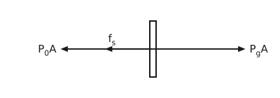
Figure 1 Forces on the piston. The piston is drawn as a narrow vertical bar seen edge on. All three forces act through its centre of mass, so all three arrows start there and lie on one horizontal line through it. One arrow points to the right, labelled \(P_{g}A\), the force the gas in the cylinder exerts on it. Two arrows point to the left along the same line: a short one labelled \(f_{s}\), the friction force, and a long one, the same length as the arrow to the right, labelled \(P_{0}A\), the force the atmosphere exerts on the other face.
The force balance on the piston is therefore
Substituting that into Equation (2), the friction and kinetic terms cancel and
Both the initial volume and the initial number of moles are zero, since the cylinder starts evacuated with the piston at the extreme left.
Therefore,
Since the valve remains open, the gas flow will stop when \(P_{f} = P_{1}\). Therefore
Substituting into Equation (3),
Solving for \(T_{f}\),
Part (b): the amount of gas
Problem 2
The Stirling cycle is shown in Figure 2. In this process the compressor and turbine, which are on the same shaft, are cooled and heated respectively, in order to operate isothermally. The heat exchanger operates isochorically, that is, at constant volume. The \(P\)-\(V\) and \(T\)-\(S\) traces of this cycle are shown in Figure 3. The properties and path are shown in Table 1.
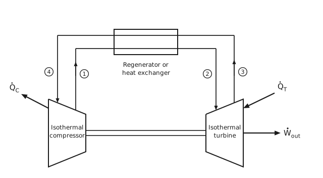
Figure 2 The Stirling cycle. An isothermal compressor on the left and an isothermal turbine on the right, drawn as trapezoids joined by a common shaft drawn as a tube, two parallel lines. A rectangle across the top is the regenerator or heat exchanger, and two stream lines cross it, one above the other. Each stream line starts and ends on the sloping top faces of the two machines. Gas leaves the compressor at state 1, rises to the lower line, crosses the regenerator from left to right, and descends into the turbine at state 2. Gas leaves the turbine at state 3, rises to the upper line, crosses the regenerator the other way, and descends into the compressor at state 4, so the two streams exchange heat as they pass. Each state number is written in a small circle beside its stream. An arrow labelled \(\dot{Q}_{C}\) leaves the compressor to the upper left, an arrow labelled \(\dot{Q}_{T}\) enters the turbine from the upper right, and an arrow labelled \(\dot{W}_{\text{out}}\) leaves the turbine to the right.
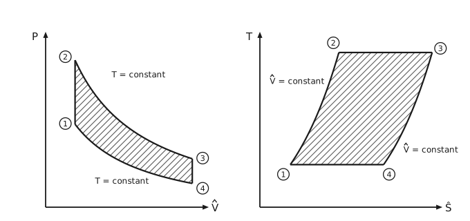
Figure 3 The Stirling cycle on pressure-volume and temperature-entropy axes. Two panels. On the left, pressure against specific volume: state 1 at the lower left and state 2 directly above it are joined by a vertical line, the constant-volume heating; a falling curve marked \(T =\) constant runs from 2 across to 3 at the right, the isothermal expansion; a short vertical line joins 3 down to 4, the constant-volume cooling; and a second falling curve marked \(T =\) constant runs from 4 back to 1. Each state number is written in a small circle. The area enclosed is hatched. On the right, temperature against specific entropy: state 1 at the lower left rises along a curve to 2 at the upper left; a horizontal line runs from 2 across to 3; a second curve falls from 3 to 4 at the lower right; and a horizontal line closes the loop from 4 back to 1. Each of the two curves is marked \(\hat{V} =\) constant just outside it, the left one to its left and the right one to its right. That area is hatched too. Both constant-volume curves bend the same way, since on constant volume the entropy goes as the logarithm of the temperature.
Point |
Path to next point |
\(T\) |
\(P\) |
\(\hat{V}\) |
\(\hat{H}\) |
Energy flow |
|---|---|---|---|---|---|---|
1 |
\(T_{1}\) |
\(P_{1}\) |
\(\hat{V}_{1}\) |
\(\hat{H}_{1}\) |
||
\(\hat{V} =\) constant |
\(\dot{Q}_{12}\) |
|||||
2 |
\(T_{2}\) |
\(P_{2}\) |
\(\hat{V}_{2} = \hat{V}_{1}\) |
\(\hat{H}_{2}\) |
||
\(\hat{T} =\) constant |
\(\dot{Q}_{T}, -\dot{W}_{23}\) |
|||||
3 |
\(T_{3} = T_{2}\) |
\(P_{3}\) |
\(\hat{V}_{3}\) |
\(\hat{H}_{3}\) |
||
\(\hat{V} =\) constant |
\(-\dot{Q}_{34} = \dot{Q}_{12}\) |
|||||
4 |
\(T_{4}\) |
\(P_{4}\) |
\(\hat{V}_{4} = \hat{V}_{3}\) |
\(\hat{H}_{4}\) |
||
\(\hat{T} =\) constant |
\(-\dot{Q}_{C}, -\dot{W}_{41}\) |
|||||
1 |
\(T_{1} = T_{4}\) |
\(P_{1}\) |
\(\hat{V}_{1}\) |
\(\hat{H}_{1}\) |
Path 1 → 2: constant volume heating
Path 2 → 3: isothermal expansion
Path 3 → 4: constant volume cooling
Path 4 → 1: isothermal compression
The efficiency of the Stirling cycle is calculated:
As \(T_{2}\) is the high temperature of the cycle and \(T_{1}\) is the low temperature, this efficiency is exactly equal to the Carnot efficiency. Indeed, it can be shown that for any cycle, if the two heat transfers to the surroundings occur at different but constant temperatures, as is the case here with an isothermal compressor and an isothermal turbine, the efficiency of the cycle will be that of a Carnot cycle.
Problem 3
Part (a): the two exit flow rates
Mark the inlet gas as A, and the exit gases as B and C. According to the mole balance:
Energy balance,
Part (b): the coldest and hottest streams a reversible tube could produce
Take the system to be the gas in the Hilsch tube, shown in Figure 4. The device is cyclic, adiabatic, and does no work.
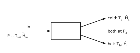
Figure 4 The Hilsch tube. A plain rectangle stands for the tube. One arrow enters it from the left, labelled “in” above it, carrying the inlet stream at \(P_{\text{in}}\), \(T_{\text{in}}\) and \(\tilde{H}_{\text{in}}\), written beneath it near its tail. Two arrows leave to the right: the upper carries the cold stream at \(T_{c}\) and \(\tilde{H}_{c}\), the lower the hot stream at \(T_{h}\) and \(\tilde{H}_{h}\), each label level with the tip of its arrow, and both discharge at the atmospheric pressure \(P_{a}\).
Take \(T_{r} = 298\) K as the enthalpy reference temperature. Then
Equation (7) turns into
Second law:
Assume \(\tilde{C}_{P} = \tfrac{7}{2}R\) and plug in numbers: \(T_{c} = 596 - T_{h}\), \(\dot{n}_{\text{in}} = 1\) mol/s, \(P_{a} = 1\) bar. We get
So if the process is reversible, the highest temperature that can be achieved is \(T_{h} = 529.09\) K, and the lowest temperature is \(T_{c} = 66.91\) K.
Problem 4
Throughout this problem, let \(Y\) be a generalized force, for example the pressure, and \(X\) the conjugate generalized displacement, for example the volume, so that
With that convention, \(W\) is the work done on the system, and a negative \(W\) therefore means work delivered to the surroundings.
(i) An isothermal and an adiabatic (reversible) cannot intersect more than once
Consider a cyclic process in which an isothermal and an adiabatic do intersect more than once, as in Figure 5.
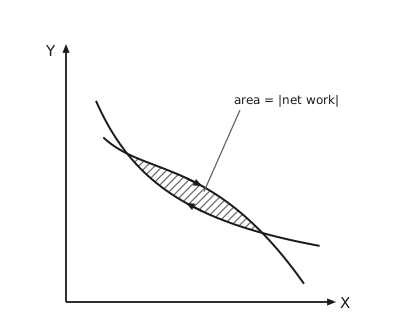
Figure 5 Two curves crossing twice. A pair of axes, the generalized force \(Y\) upward and the generalized displacement \(X\) to the right. Two falling curves leave the upper left together, separate, and meet again lower down to the right, so they enclose a narrow lens-shaped region, which is hatched and labelled by a leader line “area = |net work|”. An arrow on the upper boundary points to the right and one on the lower boundary points to the left, giving the direction the cycle is traversed. Either curve may be the isothermal and the other the adiabatic: the argument does not depend on which.
Now go around the cycle in the direction shown, so that
which is work done by the system on the surroundings. For a cyclic process,
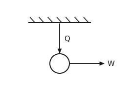
Figure 6 The device that the Kelvin-Planck statement forbids. A hatched horizontal line at the top is a single heat reservoir. An arrow labelled \(Q\) carries heat down from it into a circle, the cyclic device, and a single arrow labelled \(W\) leaves the circle to the right. There is no second reservoir, so the heat drawn from the one reservoir is converted entirely into work.
Thus we have converted heat, from a single isothermal heat reservoir, into work with no other effect, as in Figure 6. This is impossible, since it violates the Kelvin-Planck statement of the second law, and so we can conclude that an adiabat (isentrope) and an isotherm cannot intersect more than once.
Note that the above process, if run in the opposite direction, does not immediately violate the second law. Yet, since the isotherm and adiabat are reversible pathways, we are able to run the cycle in either direction, forwards or backwards. Hence impossibility in one direction automatically implies that the other direction is not possible either, that is, reversibility requires that we consider both directions in our analysis.
(ii) Two adiabatics cannot intersect
If two adiabatics are allowed to intersect, we could generate a cyclic process by connecting the two adiabatics with an isothermal, as in Figure 7.
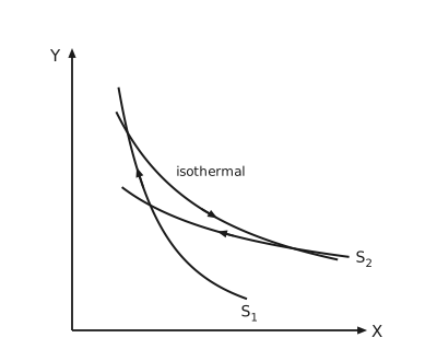
Figure 7 Two adiabatics crossing, closed by an isothermal. The same axes. Two falling curves cross near the upper left: the steeper is labelled \(S_{1}\) at its lower end and the shallower, the lower of the two long curves, \(S_{2}\) at its right-hand end. A third falling curve, labelled “isothermal”, comes down from above, cuts \(S_{1}\) near the top and crosses \(S_{2}\) near its right-hand end, so the three curves bound a closed curvilinear triangle. The arrows give the direction the cycle is traversed: down along the isothermal, back to the left along \(S_{2}\), and up along \(S_{1}\).
Taking \(S_{1}\) and \(S_{2}\) as the two adiabatics, then for the direction around the cycle shown,
So
The net effect is again the complete conversion of heat, drawn from a single isothermal source, into work, exactly the device of Figure 6. Since this is an impossibility, we conclude that two adiabatics cannot intersect.
(iii) An isothermal and an adiabatic cannot touch each other without intersecting
If the two can touch each other without intersecting, then we have a point of tangency, as in Figure 8.
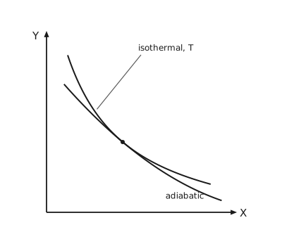
Figure 8 An isothermal and an adiabatic meeting at a point of tangency. The same axes. Two falling curves, both convex, approach each other from the upper left, meet at a single marked point, and separate again to the lower right without crossing. The adiabatic bends less than the isothermal, so it lies below it on both sides of the point. The upper curve is labelled “isothermal, \(T\)” by a leader line and the lower one “adiabatic”.
If we invoke continuity of states, then an isothermal at \(T - δT\) would intersect the adiabatic at two points, as in Figure 9, and we proceed as in part (i).
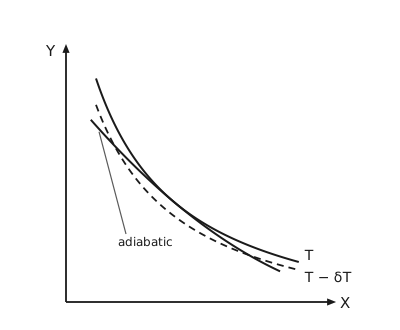
Figure 9 The isothermal displaced by a small temperature difference. The same axes again. The solid isothermal at \(T\) and the adiabatic are drawn as before, and a dashed curve lying just below the solid one is the isothermal at \(T - δT\). The dashed curve cuts the adiabatic at two separate points rather than touching it at one, which is the situation already ruled out in part (i). All three curves are convex. The two isothermals are labelled \(T\) and \(T - δT\) at their right-hand ends, and the adiabatic, which stops short of them, is labelled “adiabatic” by a leader line from the lower left.
(iv) No other heat engine operating between the same two temperatures has a higher efficiency than a reversible Carnot engine
Consider a Carnot engine operating between \(θ_{H}\) and \(θ_{C}\), as in Figure 10.
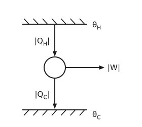
Figure 10 The reversible Carnot engine. A hatched line at the top is the reservoir at \(θ_{H}\) and a hatched line at the bottom the reservoir at \(θ_{C}\). An arrow labelled \(|Q_{H}|\) carries heat down from the hot reservoir into a circle, the engine; an arrow labelled \(|W|\) leaves the circle to the right; and an arrow labelled \(|Q_{C}|\) carries the remaining heat down into the cold reservoir.
Consider a second heat engine, operating between \(θ_{H}\) and \(θ_{C}\), and assume that it is more efficient than the Carnot engine. It is shown in Figure 11.
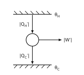
Figure 11 The second engine, assumed to be more efficient. The same arrangement as the Carnot engine: a hatched reservoir at \(θ_{H}\) above and one at \(θ_{C}\) below, with a circle between them. Its three interactions carry primes, \(|Q_{H}'|\) down into the engine, \(|W'|\) out to the right, and \(|Q_{C}'|\) down into the cold reservoir, to distinguish them from the Carnot engine’s.
Assuming \(η' > η\),
or
or
Now, run the Carnot engine in reverse. Choose its operating conditions so that if the Carnot engine were run \(n\) times in reverse, and the second engine were run \(N\) times in the forward direction, then
First law for both engines:
Subtracting the first equation from the second yields
Now
which implies that
that is, more heat is removed from \(θ_{H}\) than is added to it. This indicates that
the inequality on the right being in the sign convention set at the head of this problem, where a negative \(W\) is work delivered to the surroundings.
The net result of the total process is a transfer of heat from a single heat reservoir and its complete conversion into work, once more the device of Figure 6. This is a violation of the Kelvin-Planck statement of the second law. Hence, no other heat engine, when operating between the same two temperatures, can have a higher efficiency than a reversible Carnot engine.
A system described by three independent variables
Let the system be described by the variables \(X\), \(Y\), \(Z\), such that \(T = T(X,Y,Z)\) and \(S = S(X,Y,Z)\). The situation is drawn in Figure 12.
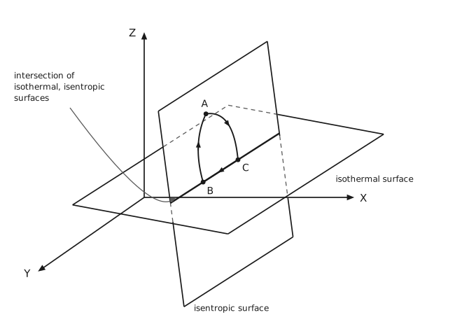
Figure 12 An isothermal surface and an isentropic surface meeting in a line. Three axes: \(Z\) upward, \(X\) to the right, and \(Y\) toward the lower left. Two flat quadrilateral patches cut through each other along a heavy straight line that climbs to the right. The nearly level one is labelled “isothermal surface” at its right. The nearly upright one, which leans so that its foot is further along \(X\) than its top, is labelled “isentropic surface” below its lowest corner. Edges of either patch that pass behind the other are dashed. The line where they meet is labelled by a curved leader from the left, “intersection of isothermal, isentropic surfaces”. Three states are marked on the isentropic surface: \(B\) and \(C\) on the line of intersection, and \(A\) above it. Arrows run from \(A\) to \(C\), along the line from \(C\) back to \(B\), and from \(B\) up to \(A\), so the cycle \(ACBA\) closes. The legs \(AC\) and \(AB\) are curves that bow outward, away from the inside of the loop. The leg \(CB\) lies on the line of intersection, so that stretch of the path is isothermal as well as isentropic.
(a) A process that is both isothermal and adiabatic (isentropic) may be realized. A process along the path \(BC\) lies in both surfaces at once, so it is both isothermal and isentropic.
(b) A cyclic process may exist in which the heat and the work each integrate to zero around the cycle. Consider the cyclic process \(ACBA\), which falls on the isentropic surface. Since \(ΔU = 0\), then
Paths \(B \to A\) and \(A \to C\) are isentropic, so \(δQ = 0\) on each; path \(C \to B\) is isentropic as well as isothermal, so \(δQ = 0\) there too. Therefore
Any cyclic process kept on the same isentropic surface satisfies the above result. Although work is performed along each path, the net work performed around the cycle is identically equal to zero.
Problem 5
Part (a): the minimum tank temperature
Take the system to be the wall unit. Write \(\dot{Q}_{h}\) for the heat it takes from the house at \(T_{h}\), \(\dot{Q}_{t}\) for the heat it takes from the tank at \(T_{t}\), and \(\dot{Q}_{s}\) for the heat it exchanges with the surrounding air at \(T_{s}\). The heat the tank supplies equals the solar influx.
First law:
Second law:
Eliminating \(\dot{Q}_{s}\) with the first law,
so the tank temperature must satisfy
Let \(γ = \dot{Q}_{h}/\dot{Q}_{t}\). Then
With \(T_{s} = 313\) K and \(T_{h} = 293\) K, the right-hand side is minimized when \(γ \to 0\), that is, when \(\dot{Q}_{t} \to \infty\). This is achieved when the collection area tends to infinity, and then
Part (b): the collection area as a function of tank temperature
From Equation (8),
The bracket on the left is negative, since \(T_{s} > T_{h}\), so dividing by it reverses the inequality.
If \(T_{t} = 323\) K, then \(S \ge 11\) m².
Part (c): should the partners invest?
The tank temperature and collector size are quite reasonable. So why not?
Problem 6
Part (a): the gamma function
The gamma function is
Integrating by parts,
or
Now show that \(Γ(n+1) = n!\) for a non-negative integer \(n\), by induction.
For \(n = 0\), so \(x = n + 1 = 1\):
\[Γ(1) = \int_{0}^{\infty} e^{-t} \cdot t^{0} \mathrm{d}t = \left. -e^{-t} \right|_{0}^{\infty} = 1 = 0!\]Assume the result for \(n = m \in \mathbb{N}\), so that \(Γ(m+1) = m!\).
For \(n = m+1\),
\[Γ(m+2) = (m+1) \cdot Γ(m+1) = (m+1) \cdot m! = (m+1)!\]
Therefore \(Γ(n+1) = n!\) for any non-negative integer \(n\).
Next, \(Γ(1/2)\):
Let \(u^{2} = t\), so that \(\mathrm{d}t = 2u \mathrm{d}u\). Then
The above result is well known and can be directly used. Or it can be derived as follows:
With \(u = r\cosθ\) and \(v = r\sinθ\),
Let \(p = r^{2}\), so \(\mathrm{d}p = 2r \mathrm{d}r\). Then
Now \(Γ(3/2)\), from the recurrence:
The general result follows by induction again.
For \(n = 1\) the line above is the statement to be proved.
Assume it for \(n = m\):
(9)¶\[Γ\left(m + \tfrac{1}{2}\right) = \frac{1 \cdot 3 \cdots (2m-1)}{2^{m}} Γ\left(\tfrac{1}{2}\right) = \frac{(2m)!}{2^{2m} \cdot m!}\sqrt{\pi}\]For \(n = m+1\),
\[Γ\left(m + 1 + \tfrac{1}{2}\right) = \left(m + \tfrac{1}{2}\right) Γ\left(m + \tfrac{1}{2}\right)\]\[= \frac{2m+1}{2} \cdot \frac{1 \cdot 3 \cdots (2m-1)}{2^{m}} Γ\left(\tfrac{1}{2}\right)\]\[= \frac{1 \cdot 3 \cdots (2m+1)}{2^{m+1}} \cdot Γ\left(\tfrac{1}{2}\right)\]
Therefore Equation (9) holds for any positive integer \(n\).
Part (b): the surface and volume of an \(N\)-dimensional sphere
The integrand factorizes, so
When \(N = 2\), in polar coordinates \(x_{1} = r\cosθ\) and \(x_{2} = r\sinθ\), so that \(\mathrm{d}x_{1}\mathrm{d}x_{2} = |J| \mathrm{d}r \mathrm{d}θ\), where \(|J|\) is the Jacobian
When \(N = 3\), in spherical coordinates \(x_{1} = r\sinθ\cosφ\), \(x_{2} = r\sinθ\sinφ\) and \(x_{3} = r\cosθ\), so
In general, writing \(I\) in hyper-spherical coordinates,
Let \(t = r^{2}\), so \(\mathrm{d}t = 2r \mathrm{d}r\). Then
According to Equation (10), \(I = \pi^{N/2}\), so
which reduces correctly in the two cases already worked out:
Finally, the volume of an \(N\)-dimensional sphere of radius \(R\):
Since \(\frac{N}{2}Γ\!\left(\frac{N}{2}\right) = Γ\!\left(\frac{N}{2}+1\right)\),
which again reduces correctly: