Properties of Pure Materials
ChE 621 — Thermodynamics.
Overview of methods for expressing thermodynamic properties
A systematic method for expressing thermodynamic properties answers the question: What needs to be measured? It should allow for
organization of data;
accuracy;
convenience;
minimum number of experiments.
In general, to construct one of the energy functions we need an \(F_{i}\)-\(x_{i}\)-\(T\) equation of state, plus \(\tilde{C}_{V}\) or \(\tilde{C}_{P}\). For example,
so we need a \(P\)-\(V\)-\(T\), a \(σ_{\mathrm{s}}\)-\(A\)-\(T\), an \(H\)-\(M\)-\(T\), an \(E\)-\(P\)-\(T\), and a \(μ_{i}\)-\(n_{i}\)-\(T\) equation of state. These are called constitutive relations, which relate state variables. They are obtained by:
empirical fitting to experimental data;
semi-empirical equations of state;
statistical mechanics and computer simulations.
Example equations of state
The \(H\)-\(M\)-\(T\) equation of state
Curie’s law for paramagnetic materials:
As shown in Figure 1, Curie’s law is the high-\(T\), low-\(H\) limit of
The Langevin paramagnetic model:
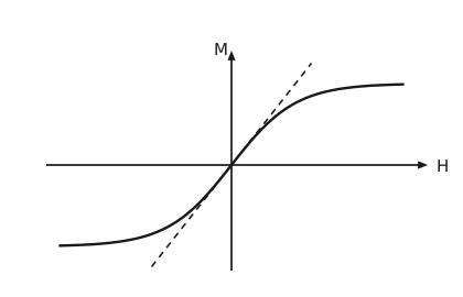
Figure 1 The Langevin magnetization curve. Magnetization \(M\) on the vertical axis against field \(H\) on the horizontal axis, both axes running through the origin so that negative fields are shown as well. The curve is an odd S-shape: it rises steeply through the origin and then flattens toward saturation, with the mirror image below for negative fields. A dashed straight line through the origin is the tangent to the curve there, and its slope is what Curie’s law gives: the law is the small-field limit of the model, and the two agree only near the origin.
The \(σ\)-\(ε\)-\(T\) equation of state
For a linear elastic material,
where \(Y\) is Young’s modulus (Figure 2).
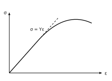
Figure 2 Stress against strain. Stress \(σ\) on the vertical axis against strain \(ε\) on the horizontal. The curve leaves the origin as a straight line, then bends over to a maximum and turns slightly down. A dashed line lies along the straight part and runs on past it: its slope is Young’s modulus, and the linear relation \(σ = Yε\) holds only while the curve and the dashed line coincide. The relation \(σ = Yε\) is written beside the upper part of the dashed line, on its left.
Wachtman’s equation, or the Mie-Grüneisen equation of state, gives the temperature dependence:
where \(Y_{0}, b_{1}\) and \(T_{0}\) are constants.
For some polymers, derived from statistical mechanics,
where \(N\) is the chain length and \(a\) is the monomer length.
The \(P\)-\(V\)-\(T\) equation of state
For an ideal gas (non-interacting, point particles),
where \(Z\) is the compressibility.
The van der Waals equation of state (Nobel Prize, 1910) is pressure-explicit:
and rearranges to a cubic equation of state:
where the two constants:
\(a\): accounts for attractive interactions;
\(b\): accounts for the finite size of molecules;
and as \(a \to 0\) and \(b \to 0\) the ideal gas is recovered. Imposing
gives
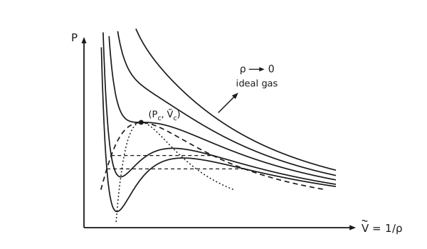
Figure 3 Van der Waals isotherms, the coexistence dome and the ideal-gas limit. Pressure on the vertical axis against molar volume, on a scale stretched at small volumes, the axis labelled \(\tilde{V} = \frac{1}{ρ}\) so it can equally be read as a reciprocal density. Five isotherms are drawn, two above the critical temperature, the critical one and two below it, unflattened, so the two subcritical ones show the characteristic loop: a steep fall on the left, a local minimum, a rise to a local maximum, then a gentle fall. A dashed horizontal tie line crosses each loop at its vapour pressure. The dashed curve through the ends of the tie lines is the coexistence dome, and it closes at the marked critical point \(\left(P_{\mathrm{c}}, \tilde{V}_{\mathrm{c}}\right)\), where the critical isotherm has a horizontal inflection. A dotted curve inside the dome is the spinodal, the locus of the turning points of the loops. Its left branch runs on below the dome, through the minimum of the coldest loop and across that isotherm, almost to the volume axis. An arrow leaves the middle of the top isotherm, rising at 45 degrees, and points at the centre of the words “\(ρ \to 0\), ideal gas”: at large volume and low density every isotherm approaches the ideal-gas hyperbola.
Isothermal compressibility and isobaric thermal expansion coefficient
A \(P\)-\(V\)-\(T\) equation of state gives \(\tilde{V}\) as a function of \(P\) and \(T\), that is \(\tilde{V}\left(P, T\right)\), or
The necessary information can also be given in the form of two coefficients, which the original brackets together:
so that
If \(β\) and \(κ\) are weak functions of \(T\) and \(P\), as they are for liquids and solids,
which is a volume-explicit equation of state.
The virial \(P\)-\(V\)-\(T\) equation of state
For the ideal gas:
The Taylor expansion of the compressibility factor around \(\tilde{ρ} = 0\), or \(\frac{1}{\tilde{V}} = 0\) gives
which gives
This is called the virial expansion, and \(B, C, D, \dots\) are called the second, third, fourth, … virial coefficients. \(B, C, D, \dots\) can be calculated using statistical mechanics.
Departure functions
For example, the residual volume is
Using the virial equation of state,
Any identity we derived also holds for the residual property. For example,
The above equation means that we can integrate from \(P \to 0\) to arbitrary \(P\), since \(\tilde{G}^{\mathrm{R}}\big|_{P=0} = 0\) at the ideal gas limit:
In general, for some property \(B\),
so that a change between two states can be assembled from three legs (Figure 4):
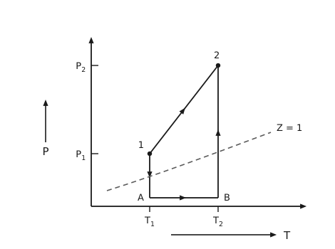
Figure 4 The path through the low-pressure limit. Pressure on the vertical axis against temperature on the horizontal, with \(P_{1}\) and \(P_{2}\) marked on one and \(T_{1}\) and \(T_{2}\) on the other. State 1 sits at \(\left(T_{1}, P_{1}\right)\) and state 2 at \(\left(T_{2}, P_{2}\right)\), joined by a straight line with an arrowhead at its middle: the direct change. Three more legs, each with an arrowhead at its middle, trace the detour: straight down from 1 to a point A just above the temperature axis, straight across from A to B at the second temperature, then straight up from B to 2. The middle leg runs at vanishing pressure, where the fluid is an ideal gas, so the residual contributions enter only on the two vertical legs. A dashed line labelled \(Z = 1\) rises across the diagram, crossing both vertical legs.
Other residual properties follow from the same route:
so that
and, since \(\tilde{S}^{\mathrm{R}} = \frac{\tilde{G}^{\mathrm{R}} - \tilde{H}^{\mathrm{R}}}{T}\),
Fugacity
For an ideal gas,
and for real fluids the pressure is replaced by the fugacity \(f\left(P,T\right)\):
Subtracting,
where the fugacity coefficient is defined as
and therefore, for a pure species, the earlier results give