Phase Equilibria of Pure Materials
ChE 621 — Thermodynamics.
One-component vapor-liquid phase equilibrium
Experiment: vary \(P\) at constant \(T\), and measure \(V\) (Figure 1)
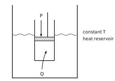
Figure 1 The compression experiment. A large vessel, open at the top, is the constant-temperature heat reservoir. Its liquid surface is drawn as a wavy line about two-fifths of the way down, on either side of a cylinder that stands in the bath. The open top of the cylinder rises above the liquid, and the fluid inside is sealed by a hatched piston that sits just below the level of the bath. A rod runs up from the piston, and beside it an arrow labelled \(P\) points down onto the piston: the pressure is imposed from outside. A curved arrow labelled \(Q\) starts in the bath below the cylinder and passes through its floor into the enclosed fluid. It shows the heat exchanged with the bath, which is what holds the temperature constant. The words “constant \(T\) heat reservoir” label the bath.
Ideal-gas PVT diagrams (Figure 2)
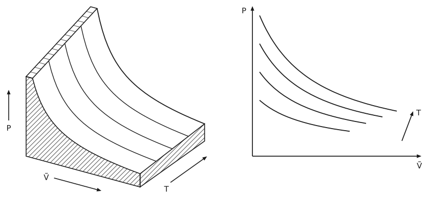
Figure 2 The ideal-gas surface and its projection. On the left, an oblique view of a solid block topped by the surface \(P = \frac{RT}{\tilde{V}}\), ruled by five isotherms. Pressure rises up the page, molar volume \(\tilde{V}\) increases toward the lower right and temperature \(T\) toward the upper right. The front face, the right-hand face and a thin strip along the back edge are hatched. The surface falls steeply as \(\tilde{V}\) grows and rises with \(T\), and it has no flat regions anywhere: an ideal gas never condenses. On the right, the same surface seen along the temperature axis, giving \(P\) against \(\tilde{V}\): four hyperbolas, one per isotherm, with an arrow beyond their ends labelled \(T\) pointing toward higher temperature.
Real fluid phase diagrams (Figure 3)
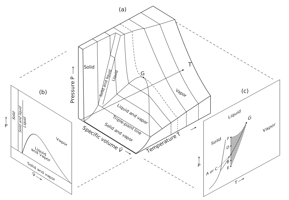
Figure 3 The PVT surface of a real fluid, with its two projections. Panel (a) is an oblique view of the surface, drawn as a solid block cut off flat at a maximum pressure. Pressure rises up the page, specific volume \(\tilde{V}\) increases toward the lower right and temperature \(T\) toward the upper right. At the smallest volumes the surface is a steep cliff labelled Solid, with a closed flat top where the cut meets it. A narrow band labelled Solid and liquid rises steeply from the triple point to the flat top, and beside it runs a narrow band labelled Liquid. Below them lies the region labelled Liquid and vapor, bounded by the coexistence dome, which closes at the marked critical point \(G\). The lowest tie line across the dome is the triple-point line, and in front of it a flat apron labelled Solid and vapor runs down to the front edge. The region to the right is labelled Vapor. Isotherms rule the surface: each crosses the flat top, comes down the cliff or the bands, crosses the dome as a straight tie line, falls along the vapor side and runs down the right-hand face of the block. Above the critical temperature the isotherms are smooth hyperbolas, as for an ideal gas. The critical isotherm, through \(G\), is dashed. An arrow drawn across the surface, labelled \(T\), points toward higher temperature. Panel (b) is the surface seen along the temperature axis, giving \(P\) against \(\tilde{V}\): narrow bands for the solid, the solid and liquid, and the liquid at the left, the dome labelled Liquid and vapor, the vapor region to the right, and a strip labelled Solid and vapor along the bottom, below the triple-point line. Panel (c) is the surface seen along the volume axis, giving \(P\) against \(T\). The sublimation curve rises from the lower left to the triple point, where the steep fusion curve and the vaporization curve leave it, and the vaporization curve ends at \(G\). The regions are labelled Solid, Liquid and Vapor. A grey band, the metastable region, rises from one isotherm to a point at \(G\), with the vaporization curve running up through it and about equal areas on either side. Both its edges are dashed and convex: the upper one bows in toward the curve near \(G\), and the lower one bulges out to the right. Five points on that isotherm are marked on a vertical line along the left of the band: \(F\) at the top, then \(D\), the point on the vaporization curve that an arrow labels “A or C”, \(B\), and \(E\) at the bottom. Panels (b) and (c) are drawn in perspective, as if on walls either side of the block, and dashed lines join them to it.
The slope of the coexistence curves in panel (c), the derivative \(\frac{\mathrm{d}P}{\mathrm{d}T}\), is derived below as the Clausius-Clapeyron equation.
Focusing on the vapor-liquid transitions, the \(p \tilde{V}\) curves at a series of temperatures are plotted in Figure 4. The simplest equations of state that can reproduce such phase transitions are cubic (i.e., having solutions for two coexisting densities, or \(\tilde{V}\), at a given pressure), such as the van der Waals equation.
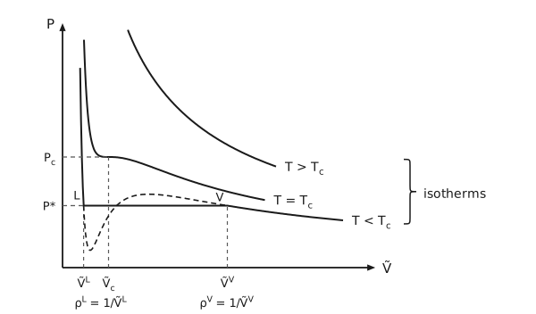
Figure 4 Isotherms above, at and below the critical temperature. Pressure on the vertical axis against molar volume on the horizontal axis. Three isotherms are drawn, each labelled at its right-hand end, from the highest, \(T > T_{\mathrm{c}}\), through \(T = T_{\mathrm{c}}\) to the lowest, \(T < T_{\mathrm{c}}\), and a curly brace beside the labels groups them as “isotherms”. All three are computed from the van der Waals equation, and on their vapor side they fall like the hyperbolas of an ideal gas. The isotherm above the critical temperature falls smoothly. The critical isotherm has a horizontal inflection at the critical point, whose pressure \(P_{\mathrm{c}}\) and volume \(\tilde{V}_{\mathrm{c}}\) are carried to the axes by dashed lines. The isotherm below the critical temperature drops steeply, runs flat at the saturjation vapor pressure \(P^{*}\) from the point labelled L to the point labelled V, and then falls away. Dashed lines carry \(P^{*}\) to the pressure axis and the volumes at L and V down to \(\tilde{V}^{\mathrm{L}}\) and \(\tilde{V}^{\mathrm{V}}\). Across the flat part the van der Waals equation itself is drawn dashed: it dips well below \(P^{*}\) just after L, rises a little above it, and rejoins at V. This loop is the part the real fluid replaces by the flat tie line. Beneath the volume axis the coexisting densities are written, \(ρ^{\mathrm{L}} = \frac{1}{\tilde{V}^{\mathrm{L}}}\) under \(\tilde{V}^{\mathrm{L}}\) and \(ρ^{\mathrm{V}} = \frac{1}{\tilde{V}^{\mathrm{V}}}\) under \(\tilde{V}^{\mathrm{V}}\).
The van der Waals equation of state
Using fitted \(a\) and \(b\) values, we can plot the \(P\)-\(V\)-\(T\) behaviour from the van der Waals equation of state, as in Figure 4. The solid-dashed line in Figure 4 and Figure 5 corresponds to a subcritical temperature. At this temperature and at pressures between E and F, solutions exist to give two coexisting density values, but how to find the correct saturation vapor pressure, \(p^{*}\)?
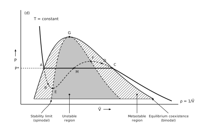
Figure 5 The metastable and unstable regions. Panel (d) of Figure 3 showing pressure against molar volume \(\tilde{V}\). The binodal, the equilibrium coexistence curve, rises from a horizontal base on the left to the critical point \(G\) and falls to the base on the right. The dashed spinodal, the stability limit, lies inside it and meets it at \(G\). The two lobes between the binodal and the spinodal are hatched: these are the metastable regions. The region inside the spinodal is shaded grey: this is the unstable region. One equilibrium isotherm, labelled \(T =\) constant, is drawn heavy: a steep liquid branch from the upper left, a horizontal tie line at the vapor pressure from \(A\) on the binodal at the left to \(C\) on the right, and the vapor branch beyond \(C\). A dashed line from the pressure axis, labelled \(P^{*}\), meets the tie line at \(A\). The van der Waals loop is drawn as dashed between the two ends of the tie line. It passes \(B\) in the left metastable lobe, reaches its minimum at \(E\) on the spinodal, rises through the unstable region, crossing the tie line at \(M\), to its maximum at \(F\) on the spinodal, and passes \(D\) in the right metastable lobe before it rejoins the tie line at \(C\). Beside the panel, an equation reads \(ρ = \frac{1}{\tilde{V}}\). Leaders below the axis label, from left to right, the stability limit or spinodal, the unstable region, the metastable region, and the equilibrium coexistence or binodal.
Route I: Maxwell equal-area construction
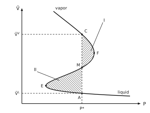
Figure 6 Molar volume against pressure, and the equal-area construction. The vertical axis is molar volume and the horizontal axis is pressure. The van der Waals isotherm, turned on its side, comes down from the upper left along the branch labelled vapor, bulges out to the right to \(F\), the highest pressure on the loop, swings back to the left to \(E\), the lowest, and then runs out to the right along the nearly flat branch labelled liquid. A dashed vertical line at the vapor pressure \(P^{*}\) rises from the pressure axis and cuts the curve three times, ending at the top one: at \(A\) on the liquid branch, at \(M\) on the middle limb and at \(C\) on the vapor branch. Dashed horizontal lines join \(C\) and \(A\) to the volume axis, where they are labelled \(\tilde{V}^{\mathrm{V}}\) and \(\tilde{V}^{\mathrm{L}}\). The area between the curve and the line on the right, from \(C\) round \(F\) to \(M\), is hatched and labelled I. The area on the left, from \(M\) round \(E\) to \(A\), is hatched the other way and labelled II. The construction sets the two areas equal.
As shown in Figure 6, the free-energy change from liquid to vapor should be zero
so that
where the left- and right-hand sides represent the areas of I and II, respectively.
Route II: the molar Gibbs energy \(\tilde{G}\left(P, T\right)\)
At constant \(T\) the temperature term drops out of
so that
Substituting the van der Waals equation,
which integrates to
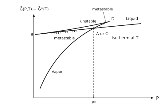
Figure 7 The molar Gibbs energy along a subcritical isotherm. The vertical axis is \(\tilde{G}\left(P,T\right) - \tilde{G}^{\circ}\left(T\right)\) and the horizontal axis is pressure. The curve, computed from the van der Waals equation, forms a swallowtail. The branch labelled Vapor rises steeply from the lower left to a cusp at \(D\). From \(D\) the branch labelled unstable runs back down to the left, just above the others, to a second cusp at \(B\). From \(B\) the nearly flat branch labelled Liquid runs to the right. The words “Isotherm at \(T\)” stand just below the right-hand end of the liquid branch. The vapor and liquid branches cross at a marked point labelled “A or C”, at the vapor pressure \(P^{*}\), from which a dashed line drops to a tick on the pressure axis: the fluid follows whichever branch lies lower, so it switches from vapor to liquid there. Short hatching along the middle of each marks the two stretches beyond the crossing, the vapor branch from the crossing up to \(D\) and the liquid branch from the crossing back to \(B\), and each is labelled metastable. The letters follow panel (c) of Figure 3.
The numerical recipe is:
Pick \(\tilde{V}\) and calculate \(P\) using the van der Waals equation of state.
Calculate \(\tilde{G}\left(P,T\right) - \tilde{G}^{\circ}\left(T\right)\).
which tabulates as
Plotting \(\tilde{G}\) against \(P\) gives Figure 7, the intersection where the liquid and vapor branches meet gives the saturation vapor pressure, \(P^{*}\).
Route III: the molar Helmholtz energy \(\tilde{A}\left(\tilde{V}, T\right)\)
At constant \(T\) the temperature term drops out of
so that
which integrates to
See Figure 8: A common tangent line finds the coexisting densities.
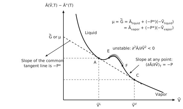
Figure 8 The molar Helmholtz energy against molar volume. The vertical axis is \(\tilde{A}\left(\tilde{V},T\right) - \tilde{A}^{\circ}\left(T\right)\) and the horizontal axis is molar volume. The curve falls steeply along the branch labelled Liquid, flattens, dips slightly, rises over a small hump and falls again along the branch labelled Vapor. A dashed common tangent touches it at \(A\) and at \(C\) and runs back to the vertical axis, where its intercept is labelled \(\tilde{G}\) or \(μ\). Dashed lines carry \(A\) and \(C\) to both axes, where they mark \(\tilde{V}^{\mathrm{L}}\) and \(\tilde{V}^{\mathrm{V}}\). The concave arc from \(E\) to \(F\), between the two inflection points, carries a comb of short strokes and is labelled “unstable: \(\partial ^{2}\tilde{A}/\partial \tilde{V}^{2} < 0\)”. An arrow from the tangent line points to the label “Slope of the common tangent line is \(-P^{*}\)”, and an arrow from the label “Slope at any point: \(\left(\partial \tilde{A}/\partial \tilde{V}\right)_{T} = - P\)” points to the curve halfway between \(F\) and \(C\). In the upper right of the plot is written \(μ = \tilde{G} = \tilde{A}_{\text{liquid}} + \left(- P^{*}\right)\left(- \tilde{V}_{\text{liquid}}\right) = \tilde{A}_{\text{vapor}} + \left(- P^{*}\right)\left(- \tilde{V}_{\text{vapor}}\right)\). The letters follow panel (c) of Figure 3.
Some notes
Fluids trace the lowest lying branch, unless metastable states can be maintained.
Connecting the equilibrium points, \((\tilde{V}^V, P^{*})\) and \((\tilde{V}^L, P^{*})\), at different temperatures gives the binodal curves in Figure 5. Applying the stability criteria, \(\partial ^{2}\tilde{A}/\partial \tilde{V}^{2} = - \partial P/\partial \tilde{V} \le 0\), the limits of stability can be identified as points E and F. Connecting these points at different temperatures gives the spinodal curves. These points are labelled accordingly in Figure 6 – Figure 8.
The critical point lies on the spinodal curve and is a maximum:
which gives
For any substance, we can therefore use its critical properties to fit \(a\) and \(b\).
\(\tilde{G}\) is continuous during a phase change, but \(\tilde{V} = \left(\frac{\partial \tilde{G}}{\partial P}\right)_{T}\) and \(\tilde{S} = - \left(\frac{\partial \tilde{G}}{\partial T}\right)_{P}\) are not (Figure 9).
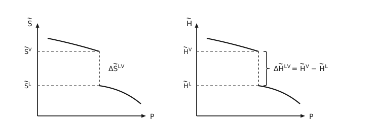
Figure 9 The entropy and the enthalpy each jump at the vapor pressure. Two panels, each plotting a molar property against pressure along one isotherm. On the left, \(\tilde{S}\): the curve falls gently along the vapor branch, drops vertically at the vapor pressure from \(\tilde{S}^{\mathrm{V}}\) to \(\tilde{S}^{\mathrm{L}}\), and continues falling, more steeply, along the liquid branch. The jump is labelled \(Δ\tilde{S}^{\text{LV}}\). On the right the same construction for \(\tilde{H}\), with a curly brace spanning the jump and the label \(Δ\tilde{H}^{\text{LV}} = \tilde{H}^{\mathrm{V}} - \tilde{H}^{\mathrm{L}}\), which is the latent heat. The vertical drop is drawn dashed in both panels, because the property is not defined between the two values, and dashed lines carry both values to the vertical axis.
Classification of phase transitions
The Ehrenfest classification (1933): defines first-order phase transitions as those in which \(\tilde{G}\), or \(\tilde{A}\), for the two phases are equal, while the derivatives with respect to \(P\) and \(T\), or with respect to \(\tilde{V}\) and \(T\), are discontinuous.
Modern classification: distinguishes first-order and continuous phase transitions by latent heat and critical scaling behavior. First-order phase transitions have a latent heat, which is the enthalpy jump \(Δ\tilde{H}^{\text{LV}} = \tilde{H}^{\mathrm{V}} - \tilde{H}^{\mathrm{L}}\) of the right-hand panel of Figure 9.
Extensive properties of a liquid-vapor mixture
For \(M = H, U, G, A\) or \(V\),
Quantifying the discontinuity: the Clausius-Clapeyron equation
How do we quantify the magnitude of the discontinuity? At coexistence the two molar Gibbs energies are equal, and so are their changes along the coexistence curve:
Writing each out,
which rearranges to
From \(\mathrm{d}\tilde{H} = T \mathrm{d}\tilde{S} + \tilde{V} \mathrm{d}P\), at the transition
or
Since \(\tilde{V}^{\mathrm{V}} \gg \tilde{V}^{\mathrm{L}}\) for \(T \ll T_{\mathrm{c}}\),
and therefore
If \(Δ\tilde{H}^{\text{LV}}\) can be considered constant over some temperature range, then integration gives \(\ln P^{*} = - \frac{Δ\tilde{H}^{\text{LV}}}{RT} + \text{constant}\). A plot of \((\frac{1}{T}, \ln P^{*})\) will give \(Δ\tilde{H}^{\text{LV}}\).
How do we get the \(T\) and \(P\) dependence of \(Δ\tilde{H}^{\text{LV}}\)? From
subtract the above expressions for the vapor and liquid phases:
Other phase equilibria in a one-component system
Solid-liquid equilibrium
Consider the plot of \(\tilde{G}\) vs. \(T\) in Figure 10. Since \(\frac{\partial \tilde{G}}{\partial T} = - \tilde{S}\), and the molar entropy of the solid is smallest and that of the vapor largest, the three branches have increasingly steep negative slopes. If the pressure is fixed at \(P = P_1\), following the lowest free-energy branch gives the melting (solid-liquid) and boiling (liquid-vapor) transitions. What happens if \(P\) is lowered? Which of the three curves moves the most?
Since \(\frac{\partial \tilde{G}}{\partial P} = \tilde{V}\), the vapor line, having the largest molar volume, is expected to move the most. The vapor line crossing the same solid-liquid intersection gives the triple point and the vapor line past the solid-liquid intersection gives the sublimation point.
Collecting the phase transition temperatures at different pressures give the \(P-T\) plot in Figure 11.
According to the Gibbs phase rule
where \(C\) is the number of components, \(P\) the number of phases, and the 2 counts \(T\) and \(P\). For a one-component system,
Therefore, a single phase represents a 2D area, two coexisting phases are constrained to a line, and three coexisting phases are a single point in the phase diagram.
Between any two phases \(α\) and \(β\), the slope
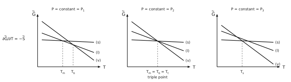
Figure 10 Three isobars that order the transition temperatures. Three panels, each plotting \(\tilde{G}\) against \(T\) at a fixed pressure, with three straight branches labelled (s) for solid, \(\left(l\right)\) for liquid and (v) for vapor. The solid branch is the flattest and the vapor branch the steepest, because the slope of each is minus that phase’s molar entropy, as \(\partial \tilde{G}/\partial T = - \tilde{S}\) written beside the first panel says. In the first panel, at \(P = P_{1}\), the branches cross at two separate temperatures, marked \(T_{\mathrm{m}}\) where solid gives way to liquid and \(T_{\mathrm{b}}\) where liquid gives way to vapor. In the second, at \(P = P_{2}\), the three branches meet at a single temperature, marked \(T_{\mathrm{m}} = T_{\mathrm{b}} = T_{\mathrm{t}}\), with the words “triple point” beneath. In the third, at \(P = P_{3}\), the solid branch crosses the vapor branch directly at the temperature marked \(T_{\mathrm{s}}\), and the liquid is never the lowest branch: the solid sublimes.
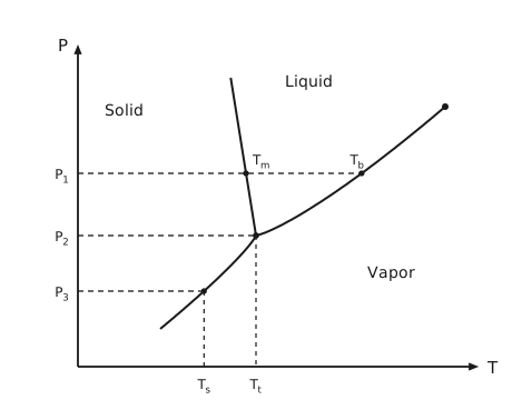
Figure 11 The pressure-temperature phase diagram. Pressure on the vertical axis against temperature on the horizontal. Three curves meet at a marked triple point: the sublimation curve rising from the lower left, the steep fusion curve going up from the triple point and leaning slightly back, and the vaporization curve running up to the right and ending at a marked critical point. The three regions are labelled Solid, Liquid and Vapor. Three dashed isobars run from the pressure axis. The highest, \(P_{1}\), crosses the fusion curve at a dot labelled \(T_{\mathrm{m}}\) and ends on the vaporization curve at a dot labelled \(T_{\mathrm{b}}\). The middle one, \(P_{2}\), ends at the triple point, and the lowest, \(P_{3}\), ends on the sublimation curve. Dashed lines drop from the triple point and from the end of \(P_{3}\) to the temperature axis, marking the triple-point temperature \(T_{\mathrm{t}}\) and the sublimation temperature \(T_{\mathrm{s}}\).
Solid-solid equilibrium
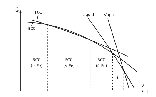
Figure 12 The Gibbs energy branches of the iron phases. A sketch of \(\tilde{G}\) against \(T\). Two gently falling branches, both bending downward, labelled FCC and BCC at the left, cross twice: BCC is lower at first, FCC is lower between the two crossings, and BCC, which bends down more steeply, is lower again after the second. Two much steeper branches, labelled Liquid and Vapor, come down from the top. The liquid branch crosses below BCC, and the vapor branch then crosses below the liquid. Dashed vertical lines drop from the four crossings and divide the temperature axis into the ranges where each phase has the lowest Gibbs energy, labelled from left to right BCC (\(α\)-Fe), FCC (\(γ\)-Fe), BCC (\(δ\)-Fe), L and V. Iron therefore changes crystal structure twice on heating before it melts.
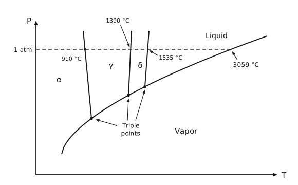
Figure 13 The iron phase diagram. Pressure against temperature. One curve, the sublimation and then the vaporization curve, rises from the lower left to the right, and a dashed horizontal line at 1 atm meets it at 3059 °C, marked by an arrow. Three steep boundaries come down from above the 1 atm line and end on the curve at three marked points, to which arrows from the words “Triple points” point. They separate the fields labelled \(α, γ\) and \(δ\), with Liquid above the curve to the right and Vapor below it. Where the boundaries cross 1 atm the transition temperatures are marked: 910 °C between \(α\) and \(γ\), 1390 °C between \(γ\) and \(δ\), and 1535 °C where \(δ\) melts.
Information one can extract from Figure 12 and Figure 13: Since \(α\)-Fe converts to \(γ\)-Fe upon heating,
and from the phase diagram
that is, \(γ\)-Fe is denser than \(α\)-Fe.
Nucleation of a gas phase in a liquid phase
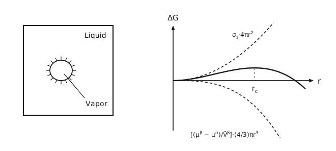
Figure 14 Nucleation of a bubble. On the left, a square vessel of liquid, labelled Liquid at the upper right, holds a small circular bubble at its centre, drawn with short radial strokes around it to mark the interface, and a leader runs from inside the bubble to the label Vapor at the lower right. On the right, the free energy change \(\Delta G\) against the bubble radius \(r\). Two dashed curves are the two competing terms: the surface term \(σ_{\mathrm{s}}\cdot 4πr^{2}\), which rises, and the volume term \(\frac{μ^{β} - μ^{α}}{\tilde{V}^{β}}\cdot \frac{4}{3}πr^{3}\), which falls away more steeply. Their sum, the heavy curve, rises to a maximum, at the critical radius, marked by a dashed vertical line down to \(r_{\mathrm{c}}\) on the axis, and then falls and crosses the axis: a bubble smaller than the critical radius shrinks, and a larger one grows.
When tracing the lowest-lying Gibbs-energy branch in the above discussions, bulk vapor and liquid phases are assumed. However, phase transitions are not instantaneous. Consider the emergence of an initial gas bubble in a parent liquid phase, with the surface term included,
Denote the amount of molecules in the gas bubble as \(\mathrm{d}N\), we have
Take the vapor bubble to be spherical, so that \(A = 4πr^{2}\) and \(\mathrm{d}N = \frac{4}{3}\,\frac{πr^{3}}{\tilde{V}^{β}}\). Then
The maximum in \(\Delta G\) can be solved, yielding the critical radius, \(r_{\mathrm{c}}\) and a free-energy barrier, which can be substituted into the rate expression of the classical nucleation theory to give the rate of homogeneous nucleation.