Thermodynamics of Non-Ideal Mixtures
ChE 621 — Thermodynamics.
Fugacity in a mixture
We begin with a two-by-two comparison. Across each row a pure gas is mixed; down each column the ideal gas gives way to the more realistic real gas.
Pure gas |
Mixture |
|
|---|---|---|
Ideal gas |
\(μ^{\text{ig}} = μ^{\circ}\left(T\right) + RT \ln P\) |
\(\begin{aligned} μ_{i}^{\text{ig}} &= μ_{i}^{\circ}\left(T\right) + RT \ln P_{i} \\ &= \underbrace{μ_{i}^{\circ}\left(T\right) + RT \ln P}_{μ_{i}^{*}\left(T, P\right)} {} + RT \ln x_{i} \quad \text{ideal-gas mixture} \end{aligned}\) |
Real gas |
\(μ = μ^{\circ}\left(T\right) + RT \ln f\) |
\(\begin{aligned} μ_{i} &= μ_{i}^{\circ}\left(T\right) + RT \ln \hat{f}_{i} \\ &\overset{?}{=} \begin{cases} \overbrace{μ_{i}^{\circ}\left(T\right) + RT \ln f_{i}^{*}}^{μ_{i}^{*}\left(T, P\right)} {} + RT \ln x_{i} & \text{ideal solutions} \\ μ_{i}^{\infty}\left(T, P\right) + RT \ln x_{i} & \text{ideal dilute solutions} \end{cases} \end{aligned}\) |
where \(\hat{f}_{i}\) is the fugacity of \(i\) in a mixture and \(f_{i}^{*}\) is the fugacity of \(i\) in the pure state.
How to compute fugacity in a mixture?
For a pure species,
We will need mixture \(P\)-\(V\)-\(T\) data. Consider mixtures at a given temperature and composition:
Subtract \(RT \mathrm{d} \ln P_{i}\) from both sides:
The term in \(\mathrm{d} \ln y_{i}\) vanishes at constant composition. Integrating from 0 to \(P\), with
and noting that as \(P \to 0\) we should have \(\hat{f}_{i} \to P_{i}\),
Ideal solution: assume the partial molar volume is the pure molar volume
Take \(\bar{V}_{i} = \tilde{V}_{i}\), which is to say \(ΔV_{\text{mixing}} = 0\), an ideal solution. Then
This is a way to calculate a mixture fugacity from the pure-component fugacity. Substituting it back,
The rule is good at:
low pressure, when the gases are nearly ideal;
any pressure when \(i\) is in excess, \(y_{i} \ge 0.9\). It is exact in the limit \(y_{i} \to 1\);
a wide range of composition when the constituents have similar physical properties: N\(_{2}\) with CO, benzene with toluene, and so on;
and it fails at high pressure when conditions 2 and 3 are not satisfied.
Non-ideal solution: evaluate the fugacity from mixture \(P\)-\(V\)-\(T\) behaviour
The problem is that empirical equations of state are not easy to generalize to mixtures. Using the van der Waals equation, for instance, how does one calculate \(a_{\text{mixture}}\) and \(b_{\text{mixture}}\) from the single-component \(a\) and \(b\) parameters? Without a way to estimate mixture parameters, one has to measure mixture \(P\)-\(V\)-\(T\) properties, potentially at many different compositions.
Consider instead the virial equation of state, which has a more sound theoretical basis. For a one-component system,
The second virial coefficient carries the two-body interactions,
with \(u\left(r\right)\) the pair potential, and the third carries the three-body interactions,
where
\(u\left(r\right)\) is often approximated by a Lennard-Jones potential (Figure 1). For pure component 1,
and similarly for component 2, with \(ε_{22}\) and \(σ_{22}\).
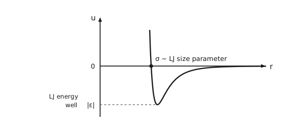
Figure 1 The Lennard-Jones pair potential. The pair potential \(u\) on the vertical axis against separation \(r\) on the horizontal, the horizontal axis crossing the vertical one at \(u = 0\), marked 0. The curve falls almost vertically from large positive values at small separation and crosses zero at a dot, where \(r = σ\). Just past the crossing, above the axis, is written \(σ \sim\) LJ size parameter, LJ standing for Lennard-Jones: \(σ\) is the separation where \(u\) is zero. The curve continues down to a single minimum and then rises back toward zero from below as the separation grows. A dashed horizontal line runs from the vertical axis to the minimum, and where it meets the axis the depth is marked \(|ε|\), like a tick label, with LJ energy well written to its left. The two parameters of the model are therefore read directly off the curve: \(σ\) where it crosses zero and \(ε\) at its deepest point.
For a mixture of 1 and 2 we need, in addition, the cross parameters
and with them
Therefore
One can show that the mixture second virial coefficient is the composition-weighted sum
Therefore one can calculate virial parameters from the knowledge of molecular interactions of pure components only (through \(\epsilon_{\mathrm{aa}}\), \(\sigma_{\mathrm{bb}}\), and so on). Many correlations for \(B\) were developed; for example, the Pitzer corresponding-states correlation:
with mixture critical properties, each of which mirrors one of the cross-parameter rules above:
and with the reduced temperature \(T_{\mathrm{r}} = \frac{T}{T_{\mathrm{c}}}\).
Non-ideal solution: excess properties and activity coefficients
An excess property is the difference between the actual property and the ideal-solution value at the same \(T, P\) and composition:
By differentiation with respect to \(n_{i}\) we have partial molar excess properties:
Applied to the chemical potential, the two references are
and their difference defines the activity coefficient:
Equivalently, in terms of the activity \(a_{i}\),
For an ideal solution \(\hat{f}_{i} = x_{i} f_{i}^{*}\), the Lewis-Randall rule, so \(γ_{i} = 1\) and \(\bar{G}^{\mathrm{E}} = 0\).
The calculus of excess properties is identical to that of molar or partial molar properties.
The temperature and pressure dependence of \(γ_{i}\) is given by
Since \(\tilde{M} = \sum x_{i} \bar{M}_{i}\) for any property,
and the Gibbs-Duhem equation at constant \(T\) and \(P\) gives
Experimental measurement of excess properties and fugacity
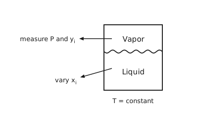
Figure 2 Measuring activity coefficients. A closed vessel divided by a wavy horizontal interface, the upper region labelled Vapor and the lower Liquid. Two arrows start inside the vessel and leave through its left wall: the one from the vapor points to measure \(P\) and \(y_{i}\), and the one from the liquid points down to the left, to vary \(x_{i}\). Below the vessel, \(T =\) constant. One isothermal series of such measurements is what Table 2 and Table 3 report.
The above relationships provide the basis for measuring the following quantities experimentally: \(\bar{V}_{i}^{\mathrm{E}}\) and \(\bar{H}_{i}^{\mathrm{E}}\), from mixing experiments, and \(γ_{i}\), from vapor-liquid equilibria. Consider phase equilibrium experiments at low pressure (Figure 2):
But \(f_{i}^{\mathrm{L}} = f_{i}^{\mathrm{V}}\), and for an ideal vapor \(f_{i}^{\mathrm{L}} = P_{i}^{\text{sat}}\), so
In Table 2 and Table 3, the first row is the pure second component and the last row the pure first component. An em dash marks a quantity that is indeterminate at that end of the composition range; the last column is left empty on the two pure-component rows for the same reason.
The chloroform / 1,4-dioxane mixture
The first pressure, 15.79 kPa, is \(P_{2}^{\text{sat}}\) and the last, 69.36 kPa, is \(P_{1}^{\text{sat}}\). Every activity coefficient is less than one, so this system shows negative deviations from Raoult’s law. The data are listed in Table 2 and plotted in Figure 3 and Figure 4.
\(P/\) kPa |
\(x_{1}\) |
\(y_{1}\) |
\(\ln γ_{1}\) |
\(\ln γ_{2}\) |
\(\frac{G^{\mathrm{E}}}{RT}\) |
\(\frac{G^{\mathrm{E}}}{x_{1}x_{2}RT}\) |
|---|---|---|---|---|---|---|
15.79 |
0.0000 |
0.0000 |
— |
0.000 |
0.000 |
|
17.51 |
0.0932 |
0.1794 |
−0.722 |
0.004 |
−0.064 |
−0.758 |
18.15 |
0.1248 |
0.2383 |
−0.694 |
−0.000 |
−0.086 |
−0.790 |
19.30 |
0.1757 |
0.3302 |
−0.648 |
−0.007 |
−0.120 |
−0.825 |
19.89 |
0.2000 |
0.3691 |
−0.636 |
−0.007 |
−0.133 |
−0.828 |
21.37 |
0.2626 |
0.4628 |
−0.611 |
−0.014 |
−0.171 |
−0.882 |
24.95 |
0.3615 |
0.6184 |
−0.486 |
−0.057 |
−0.212 |
−0.919 |
29.82 |
0.4750 |
0.7552 |
−0.380 |
−0.127 |
−0.248 |
−0.992 |
34.80 |
0.5555 |
0.8378 |
−0.279 |
−0.218 |
−0.252 |
−1.019 |
42.10 |
0.6718 |
0.9137 |
−0.192 |
−0.355 |
−0.245 |
−1.113 |
60.38 |
0.8780 |
0.9860 |
−0.023 |
−0.824 |
−0.120 |
−1.124 |
65.39 |
0.9398 |
0.9945 |
−0.002 |
−0.972 |
−0.061 |
−1.074 |
69.36 |
1.0000 |
1.0000 |
0.000 |
— |
0.000 |
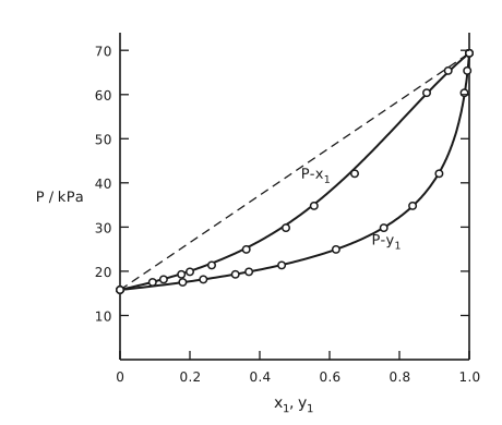
Figure 3 Pressure against composition for chloroform (1) with 1,4-dioxane (2) at 50 °C. Pressure in kilopascals on the vertical axis, from 0 to about 74 and ticked every 10, against \(x_{1}\) and \(y_{1}\) from 0 to 1 on the horizontal. The frame is open at the top: the bottom axis, the left axis, and a right axis at \(x_{1} = 1\) with the same ticks as the left one but no numbers. Two smooth curves join the two pure-component saturation pressures, 15.79 kilopascals at the left edge and 69.36 at the right, and both carry open circles, the measured points of Table 2. The upper curve, labelled \(P\)-\(x_{1}\) above and to its left, is pressure against liquid composition, the bubble line. The lower curve, labelled \(P\)-\(y_{1}\) below and to its right, is pressure against vapor composition, the dew line. A long-dashed straight line between the two ends is the line Raoult’s law would give. Both curves lie below that line across the whole range, which is what a negative deviation looks like: the mixture holds on to its molecules more tightly than an ideal solution would. The curves are the Margules correlation of the next section, with \(A_{12} = −0.72\) and \(A_{21} = −1.27\), and the circles scatter slightly about them.
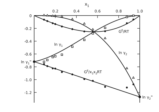
Figure 4 Liquid-phase properties from the VLE data for chloroform (1) with 1,4-dioxane (2) at 50 °C. The composition axis \(x_{1}\) runs along the top of the frame from 0 to 1, and the vertical scale runs downward from 0 to about −1.36, ticked every 0.2. The frame is the top axis, the left axis, and a right axis at \(x_{1} = 1\) with the same ticks as the left one but no numbers. Each quantity has its own marker, scattered about a smooth curve. Open squares: \(\ln γ_{1}\), whose curve starts at −0.72 at the left and rises to zero at the right, where species 1 is pure. Open triangles: \(\ln γ_{2}\), zero at the left and falling ever more steeply to −1.27 at the right. Filled circles on the upper of the two remaining curves: \(\frac{G^{\mathrm{E}}}{RT}\), a shallow trough with its minimum near −0.25 at about \(x_{1} = 0.55\), crossing the other two curves there. Filled circles on the lower one: \(\frac{G^{\mathrm{E}}}{x_{1}x_{2}RT}\), which is drawn as a straight line from −0.72 at the left edge to −1.27 at the right. Its two ends are marked with dots and labelled outside the frame, \(\ln γ_{1}^{\infty}\) beyond the left axis and \(\ln γ_{2}^{\infty}\) beyond the right one: they are the two limiting activity coefficients, and the curves for \(\ln γ_{1}\) and \(\ln γ_{2}\) start from them. That straight line is the observation the Margules equations of the next section are built on, and all four curves are those equations with \(A_{12} = −0.72\) and \(A_{21} = −1.27\).
The methyl ethyl ketone / toluene mixture
Here \(P_{2}^{\text{sat}} = 12.30\) kPa and \(P_{1}^{\text{sat}} = 36.09\) kPa, and the activity coefficients are greater than one, so this system shows positive deviations. The data are listed in Table 3 and plotted in Figure 5 and Figure 6.
\(P/\) kPa |
\(x_{1}\) |
\(y_{1}\) |
\(\ln γ_{1}\) |
\(\ln γ_{2}\) |
\(\frac{G^{\mathrm{E}}}{RT}\) |
\(\frac{G^{\mathrm{E}}}{x_{1}x_{2}RT}\) |
|---|---|---|---|---|---|---|
12.30 |
0.0000 |
0.0000 |
— |
0.000 |
0.000 |
|
15.51 |
0.0895 |
0.2716 |
0.266 |
0.009 |
0.032 |
0.389 |
18.61 |
0.1981 |
0.4565 |
0.172 |
0.025 |
0.054 |
0.342 |
21.63 |
0.3193 |
0.5934 |
0.108 |
0.049 |
0.068 |
0.312 |
24.01 |
0.4232 |
0.6815 |
0.069 |
0.075 |
0.072 |
0.297 |
25.92 |
0.5119 |
0.7440 |
0.043 |
0.100 |
0.071 |
0.283 |
27.96 |
0.6096 |
0.8050 |
0.023 |
0.127 |
0.063 |
0.267 |
30.12 |
0.7135 |
0.8639 |
0.010 |
0.151 |
0.051 |
0.248 |
31.75 |
0.7934 |
0.9048 |
0.003 |
0.173 |
0.038 |
0.234 |
34.15 |
0.9102 |
0.9590 |
−0.003 |
0.237 |
0.019 |
0.227 |
36.09 |
1.0000 |
1.0000 |
0.000 |
— |
0.000 |
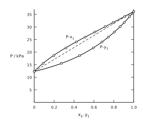
Figure 5 Pressure against composition for methyl ethyl ketone (1) with toluene (2) at 50 °C. The same layout as Figure 3: pressure in kilopascals on the vertical axis, from 0 to about 37 and ticked every 5, against \(x_{1}\) and \(y_{1}\) on the horizontal, two smooth curves with open circles, labelled \(P\)-\(x_{1}\) for the bubble line and \(P\)-\(y_{1}\) for the dew line, and a long-dashed straight Raoult’s law line between the saturation pressures 12.30 and 36.09 kilopascals. This time the bubble line lies above the dashed line across the whole range, the signature of a positive deviation, and the dew line below it. The curves are the Margules correlation with \(A_{12} = 0.372\) and \(A_{21} = 0.198\).
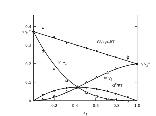
Figure 6 Liquid-phase properties from the VLE data for methyl ethyl ketone (1) with toluene (2) at 50 °C. The composition axis \(x_{1}\) runs along the bottom, from 0 to 1, and the vertical scale runs upward from 0 to about 0.46, ticked at 0.1, 0.2, 0.3 and 0.4. The frame is the bottom axis, the left axis, and a right axis at \(x_{1} = 1\) with the same ticks as the left one but no numbers. The markers are those of Figure 4, and everything is its mirror with the signs reversed. Open squares: \(\ln γ_{1}\), whose curve falls from 0.372 at the left to zero at the right. Open triangles: \(\ln γ_{2}\), rising from zero to 0.198. Filled circles on the lower curve: \(\frac{G^{\mathrm{E}}}{RT}\), a shallow arch peaking near 0.072 at about \(x_{1} = 0.42\), where the curves for \(\ln γ_{1}\) and \(\ln γ_{2}\) cross it. Filled circles on the upper one: \(\frac{G^{\mathrm{E}}}{x_{1}x_{2}RT}\), again drawn as a straight line, from 0.372 at the left edge to 0.198 at the right. Its two ends are marked with dots and labelled outside the frame, \(\ln γ_{1}^{\infty}\) beyond the left axis and \(\ln γ_{2}^{\infty}\) beyond the right one. The first point of that column, 0.389, sits above the line at the left, and at the right the last triangle, 0.237, and the last filled circle, 0.227, sit above both curves.
Margules equations
The observation in Figure 4 and Figure 6 is that \(\frac{\tilde{G}^{\mathrm{E}}}{x_{1}x_{2}RT}\) is linear with composition:
\(A_{12}\) and \(A_{21}\) are the Margules coefficients. They can be obtained from the slope and the intercepts of a plot of \(\frac{\tilde{G}^{\mathrm{E}}}{x_{1}x_{2}RT}\) against \(x_{1}\), which is exactly the near-straight line drawn in each of those two figures. Rearranging,
and since
we get the Margules equations:
with the temperature dependence carried in
Regular and athermal solution theories
It turns out that the Margules equations correspond to regular solution theories, which are all right for molecules with similar sizes and similar internal degrees of freedom of the enthalpy. There, in
the excess entropy \(\tilde{S}^{\mathrm{E}}\) is zero, so that
The other scenario, where \(\tilde{H}^{\mathrm{E}} = 0\),
gives athermal solution theories, and the Flory-Huggins model, developed below, is one of them.
Flory-Huggins model, with no interactions
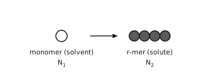
Figure 7 The two species of the lattice model. On the left a single open circle, labelled monomer (solvent), \(N_{1}\). An arrow leads to the right, to four shaded circles touching in a row, labelled \(r\)-mer (solute), \(N_{2}\). The solute is a chain of \(r\) segments, each the size of one solvent molecule, and that size difference is the whole content of the model.
We will first assume \(\tilde{H}^{\mathrm{E}} = 0\) (i.e., an athermal solution) and relax this assumption later. This assumption can describe polymers dissolved in the solvent consisting of its monomers (e.g., polystyrene / ethylbenzene; see Figure 7).
Consider a 2-dimensional lattice model with a coordination number of \(Z = 4\). There are \(N\) available sites, of which \(N_1\) are occupied by the solvent and \(rN_{2}\) are occupied by polymer:
Boltzmann’s entropy formula
requires counting \(Ω_{\text{mixture}}\), the number of configurations in which \(N_{1}\) monomers and \(N_{2}\) \(r\)-mers can be arranged in \(N\) locations (Figure 8).
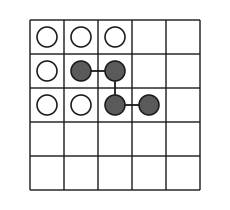
Figure 8 The lattice. A five by five square grid. Six cells hold a single open circle each, the monomer solvent: the first three cells of the top row and the first cell of the second row, and the first two cells of the third row. Four shaded circles joined in sequence by a line are one \(r\)-mer occupying four adjacent sites: the second and third cells of the second row, then down to the third cell of the third row and across to the fourth. The rest of the grid, including the bottom two rows, is empty. The counting argument that follows is the number of ways of placing \(N_{1}\) monomers and \(N_{2}\) chains on such a grid.
Let us place the polymers first. Consider the \(\left(i+1\right)\)-th polymer. With \(i\) chains already placed, \(N - ir\) sites are still available, so
The Flory-Huggins model assumes the fraction of vacant sites next to a bead is the same as the average for the entire lattice.
where the product is the falling factorial
Once the polymers are placed, there are \(N_1\) vacant sites to place the monomers, for a total of \(\frac{N_{1}!}{N_{1}!} = 1\) distinct configuration.
Therefore
For pure solvent, \(N_{2} = 0\) and \(N = N_{1}\), so \(S_{1} = S_{\text{mixture}} = 0\). For pure polymer,
Therefore the whole second bracket cancels in the difference, and
If the solvent and the monomer have similar molecular sizes, then we can interpret
as volume fractions. Using \(R = k_{\mathrm{B}} N_{\mathrm{A}}\), \(N = N_{1} + rN_{2}\), \(x_{1} = \frac{N_{1}}{N}\) and \(x_{2} = \frac{N_{2}}{N}\),
This result can be compared with
Note that \(r \to 1\) gives back the ideal solution. The excess entropy is
and, with no enthalpy of mixing,
Flory-Huggins theory that takes interactions into account
Here \(χ\) is the Flory-Huggins interaction parameter, or \(χ\)-parameter. The activity coefficient of the solvent is
P. J. Flory, J. Chem. Phys. 1941, 9, 660; 1942, 10, 51.
M. L. Huggins, J. Chem. Phys. 1941, 9, 440.
P. J. Flory, Principles of Polymer Chemistry, 1953.
van Laar model
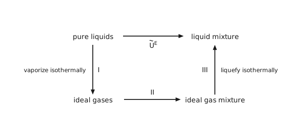
Figure 9 The van Laar path. Four states at the corners of a rectangle. Top left, pure liquids; top right, liquid mixture; bottom left, ideal gases; bottom right, ideal gas mixture. The quantity wanted, \(\tilde{U}^{\mathrm{E}}\), is the arrow straight across the top from pure liquids to liquid mixture. It is computed instead along three arrows: step I straight down the left side, vaporize isothermally; step II across the bottom, from ideal gases to ideal gas mixture; step III straight up the right side, liquefy isothermally. The middle step costs nothing because ideal gases do not interact, so the whole excess energy comes from the two vertical legs.
Consider a binary mixture with molar fractions of \(x_{1}\) and \(x_{2}\). The van Laar model makes two assumptions:
no volume change, \(V^{\mathrm{E}} = 0\);
the entropy of mixing is given by the ideal solution, \(S^{\mathrm{E}} = 0\).
Then the excess Gibbs energy is the excess internal energy:
which the model computes along a three-step path (Figure 9).
Step I. From the van der Waals equation of state,
Integrating for both components in the mixture,
where van Laar further took \(\tilde{V}^{\mathrm{L}} ≃ b\).
Step II. \(Δ\tilde{U}_{\text{II}} = 0\).
Step III.
which needs mixing rules:
Collecting the three steps,
Define
with activity coefficients
and, by construction, \(S^{\mathrm{E}} = 0\) and \(V^{\mathrm{E}} = 0\).
Hildebrand-Scatchard theory, “THE” regular solution theory
Define the cohesive energy density, an energy per unit volume,
Then for a binary mixture
Define the volume fractions
so that the above expression becomes
and therefore
Hildebrand assumed the geometric-mean cross term, in the same spirit as \(ε_{12} = \sqrt{ε_{11} ε_{22}}\) earlier:
which collapses the bracket to a perfect square:
where the solubility parameters are introduced
\(\tilde{S}^{\mathrm{E}} = 0\) and \(\tilde{G}^{\mathrm{E}} = \tilde{U}^{\mathrm{E}}\)
The activity coefficients are
Notes about the solubility parameters and the Hildebrand-Scatchard theory:
\(δ\) is weakly temperature-dependent, and therefore \(\ln γ_{i} \propto \frac{1}{T}\).
The difference in \(δ\) between the mixture components provides a measure of solution non-ideality;
If we set \(r = \frac{\tilde{V}_{\text{polymer}}}{\tilde{V}_{\text{solvent}}}\), one can relate the Flory-Huggins parameter to it, \(χ_{\text{FH}} = \frac{\tilde{V}_{1}}{RT}\left(δ_{1} - δ_{2}\right)^{2}\). For good solubility, \(χ_{\text{FH}} \approx 0\) and \(δ_{1} ≃ δ_{2}\).
The theory is related to the van Laar model through
It is not good for two cases, each of which has its own family of models:
Species of different sizes, which is what Flory-Huggins is for;
Polar molecules, for which there are Wilson, NRTL, and UNIQUAC or UNIFAC.
H. Burrell, “Solubility Parameter Values”, Polymer Handbook, 1975.
Hansen and Beerbower, “Solubility Parameters”, Encyclopedia of Chemical Technology, 1971.