Homework 3 Solutions

ChE 621 — Thermodynamics.

Problem 1

Part (a): the stress in terms of isothermal derivatives

\[\mathrm{d}U = T \mathrm{d}S + V_{0} σ \mathrm{d}ε\]

At constant \(T\), divide by \(\mathrm{d}ε\):

\[\left(\frac{\partial U}{\partial ε}\right)_{T} = T \left(\frac{\partial S}{\partial ε}\right)_{T} + V_{0} σ\]

Part (b): reading the two contributions from the stress-temperature data

Define the first Legendre transform \(A = U - TS\). We have

\[\mathrm{d}A = -S \mathrm{d}T + V_{0} σ \mathrm{d}ε\]

The corresponding Maxwell relation is

\[\left(\frac{\partial S}{\partial ε}\right)_{T} = -V_{0} \left(\frac{\partial σ}{\partial T}\right)_{ε}\]

So on the constant-\(ε\) plot of \(σ\) against \(T\), the tangent has the slope

\[k = \left(\frac{\partial σ}{\partial T}\right)_{ε} = -\frac{1}{V_{0}} \left(\frac{\partial S}{\partial ε}\right)_{T}\]

The tangent line

\[σ = kT + b = -\frac{T}{V_{0}} \left(\frac{\partial S}{\partial ε}\right)_{T} + b\]

matches Equation (1) at the point \((T, σ)\). We can therefore identify the intercept

\[b = \frac{1}{V_{0}} \left(\frac{\partial U}{\partial ε}\right)_{T}\]

Part (c): a stress proportional to temperature

\(σ = cT\), that is, \(b = 0\): there is no energetic contribution. The elastic response is all due to the change in entropy.

Problem 2

Part (a): an energy function of \(T\) and \(M\)

\[\mathrm{d}U = δQ + δW = T \mathrm{d}S + μ_{0} V H \mathrm{d}M, \qquad U = f_{U}(S, M)\]
\[A = U - TS, \qquad \mathrm{d}A = \mathrm{d}U - T \mathrm{d}S - S \mathrm{d}T = -S \mathrm{d}T + μ_{0} V H \mathrm{d}M \implies A = f_{A}(T, M)\]
\[\left(\frac{\partial A}{\partial T}\right)_{M} = -S, \qquad \left(\frac{\partial A}{\partial M}\right)_{T} = μ_{0} V H\]

The Maxwell relation is

\[-\left(\frac{\partial S}{\partial M}\right)_{T} = μ_{0} V \left(\frac{\partial H}{\partial T}\right)_{M}\]

Part (b): the entropy change

\[\mathrm{d}S = \left(\frac{\partial S}{\partial T}\right)_{M} \mathrm{d}T + \left(\frac{\partial S}{\partial M}\right)_{T} \mathrm{d}M = \left(\frac{\partial S}{\partial T}\right)_{M} \mathrm{d}T - μ_{0} V \left(\frac{\partial H}{\partial T}\right)_{M} \mathrm{d}M \]

using the Maxwell relation from part (a). At fixed \(M\),

\[= \frac{1}{T} C_{V,M} \mathrm{d}T - μ_{0} \cdot V \cdot \frac{M}{c} \mathrm{d}M\]
\[S(1 \to 2) = \int_{T_{1}}^{T_{2}} \frac{1}{T} C_{V,M} \mathrm{d}T - μ_{0} \frac{V}{c} \int_{M_{1}}^{M_{2}} M \mathrm{d}M\]
\[= C_{V,M} \ln\left(\frac{T_{2}}{T_{1}}\right) - μ_{0} \frac{V}{c} \cdot \frac{1}{2}\left(M_{2}^{2} - M_{1}^{2}\right)\]

Parts (c) and (d): the lowest possible final temperature

For a reversible adiabatic demagnetization process,

\[ΔS = 0 \implies m C_{V,M} \ln\left(\frac{T_{2}}{T_{1}}\right) = μ_{0} \frac{V}{c} \cdot \frac{1}{2}\left(0 - \frac{c^{2} H^{2}}{T_{1}^{2}}\right)\]
\[T_{2} = T_{1} \times \exp\left[\frac{μ_{0}}{C_{V,M}} \frac{V}{c \cdot m} \cdot \frac{1}{2}\left(-\frac{c^{2} H^{2}}{T_{1}^{2}}\right)\right]\]
\[= 3 \times \exp\left[\frac{1.256 \times 10^{-6}}{3.9} \times \frac{(0.1)^{3}}{1.71} \cdot \frac{1}{2} \cdot \left(-\frac{5.58 \cdot \left(2.389 \times 10^{5}\right)^{2}}{9}\right)\right]\]
\[= 3 \times \exp\left[-3.33\right] = 0.11 \text{ K}\]

Part (e): the comparison with an expanding ideal gas

The Curie equation of state (\(M\)-\(H\)-\(T\)) is just like the ideal-gas equation of state. In the adiabatic process (expansion and demagnetization), \(\mathrm{d}S\) will be zero, and both the \(-P \mathrm{d}V\) term and the \(μ_{0} V H \mathrm{d}M\) term will lead to a decrease of the internal energy, which will lead to a decrease of the temperature. Thus, this cooling method is similar to the adiabatic expansion of an ideal gas.

Problem 3

\[v_{s}^{2} = \left(\frac{\partial P}{\partial ρ}\right)_{\tilde{S}} = -\frac{V^{2}}{M} \left(\frac{\partial P}{\partial V}\right)_{\tilde{S}}, \quad \text{where } ρ = \frac{M}{V}\]
\[\left(\frac{\partial P}{\partial V}\right)_{\tilde{S}} = \left(\frac{\partial P}{\partial T}\right)_{\tilde{S}} \left(\frac{\partial T}{\partial V}\right)_{\tilde{S}}\]

From the triple product rule, we know that

(2)\[\left(\frac{\partial P}{\partial T}\right)_{\tilde{S}} = -\left(\frac{\partial S}{\partial T}\right)_{P} \cdot \left(\frac{\partial P}{\partial S}\right)_{T}\]
(3)\[\left(\frac{\partial V}{\partial T}\right)_{\tilde{S}} = -\left(\frac{\partial S}{\partial T}\right)_{V} \cdot \left(\frac{\partial V}{\partial S}\right)_{T}\]

Also,

\[\mathrm{d}G = -S \mathrm{d}T + V \mathrm{d}P\]

Recall the Maxwell relation

(4)\[-\left(\frac{\partial S}{\partial P}\right)_{T} = \left(\frac{\partial V}{\partial T}\right)_{P} \quad \text{and} \quad C_{P} = T \left(\frac{\partial S}{\partial T}\right)_{P}\]

Substitute Equation (4) into Equation (2):

(5)\[\left(\frac{\partial P}{\partial T}\right)_{\tilde{S}} = -\frac{C_{P}}{T} \left(-\frac{\partial T}{\partial V}\right)_{P}\]

Recall

\[\mathrm{d}A = -S \mathrm{d}T - P \mathrm{d}V\]

and its Maxwell relation

(6)\[-\left(\frac{\partial S}{\partial V}\right)_{T} = -\left(\frac{\partial P}{\partial T}\right)_{V} \quad \text{and} \quad C_{V} = T \left(\frac{\partial S}{\partial T}\right)_{V}\]

Substitute Equation (6) into Equation (3):

(7)\[\left(\frac{\partial V}{\partial T}\right)_{\tilde{S}} = -\frac{C_{V}}{T} \left(\frac{\partial T}{\partial P}\right)_{V}\]

Thus,

\[v_{s}^{2} = -\frac{V^{2}}{M} \left(\frac{\partial P}{\partial T}\right)_{\tilde{S}} \left(\frac{\partial T}{\partial V}\right)_{\tilde{S}} = -\frac{V^{2}}{M} \left(\frac{C_{P}}{T}\right) \left(\frac{\partial T}{\partial V}\right)_{P} \left(-\frac{T}{C_{V}}\right) \left(\frac{\partial P}{\partial T}\right)_{V}\]
\[= \frac{V^{2}}{M} \frac{C_{P}}{C_{V}} \cdot \frac{\left(\partial P / \partial T\right)_{V}}{\left(\partial V / \partial T\right)_{P}}\]

This result is acceptable. Alternatively, using the triple product rule, \(\left(\frac{\partial T}{\partial V}\right)_{P} \left(\frac{\partial P}{\partial T}\right)_{V} = -\left(\frac{\partial P}{\partial V}\right)_{T}\), so

\[v_{s}^{2} = -\frac{V^{2}}{M} \frac{C_{P}}{C_{V}} \left(\frac{\partial P}{\partial V}\right)_{T}\]

Therefore, if we have a \(P\)-\(V\)-\(T\) equation of state, for example, assuming air behaves like ideal gas (\(PV = nRT\)),

\[\left(\frac{\partial P}{\partial T}\right)_{V} = \frac{nR}{V}, \qquad \left(\frac{\partial V}{\partial T}\right)_{P} = \frac{nR}{P}\]

then with \(C_{P} = 7/2 R\) and \(C_{V} = 5/2 R\) for diatomics and \(M = 29\) g/mol, we can obtain the speed of sound:

\[ v_{s} = \sqrt{\frac{V^2}{M} \frac{7/2 R}{5/2 R} \frac{nR/V}{nR/P}} = \sqrt{\frac{7PV}{5M}} \]
\[ = \sqrt{\frac{7RT}{5M}} = 346 \quad \text{m/s} \]

at \(T = 298\) K, almost spot on.

Problem 4

Take as the system a thin slab of the pipe, between section 1 at \(x\) and section 2 at \(x + \mathrm{d}x\), as in Figure 1.
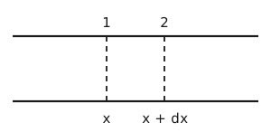
Two horizontal lines form the walls of a pipe. Two dashed vertical lines across it mark a thin slab, the left one labelled 1 above and x below, the right one labelled 2 above and x plus d x below.

Figure 1 A slab of the pipe. Two long horizontal lines are the walls of a straight pipe. Two dashed vertical lines cross the pipe from wall to wall, close together, and mark off a thin slab of it. The left one is labelled 1 above the pipe and \(x\) below it, and the right one is labelled 2 above and \(x + \mathrm{d}x\) below.

The energy balance on the slab is

and the mass balance is

(9)\[\dot{m}_{1} = \dot{m}_{2}\]

Equation (8) and Equation (9) show that

\[H + \frac{v^{2}}{2} = \text{const.}\]
\[\therefore\; \mathrm{d}H + \frac{1}{2} \cdot 2 \cdot v \cdot \mathrm{d}v = 0\]

or

\[\boxed{\mathrm{d}H = -v \mathrm{d}v}\]

Equation (9) means that

\[\dot{m} = \frac{\mathrm{d}m}{\mathrm{d}t} = ρ \cdot v \cdot A = \text{const.}\]
\[\therefore\; \mathrm{d}(ρ v A) = A \mathrm{d}\left(\frac{v}{\hat{V}}\right) = 0\]
\[\therefore\; \frac{\mathrm{d}v}{\hat{V}} - v \cdot \frac{\mathrm{d}\hat{V}}{\hat{V}^{2}} = 0\]

or

\[\boxed{\frac{\mathrm{d}v}{v} = \frac{\mathrm{d}\hat{V}}{\hat{V}}}\]

The entropy balance is

Equation (9) and Equation (10) give

\[\mathrm{d}\hat{S} = \hat{S}_{2} - \hat{S}_{1} = \frac{\dot{S}_{\text{gen}}}{\dot{m}_{1}} \ge 0\]
\[\mathrm{d}\hat{H} = T \mathrm{d}\hat{S} + \hat{V} \mathrm{d}P\]
\[\implies \mathrm{d}\hat{S} = \frac{\mathrm{d}\hat{H} - \hat{V} \mathrm{d}P}{T} \ge 0\]
\[\therefore\; \mathrm{d}\hat{H} - \hat{V} \mathrm{d}P = -v \mathrm{d}v - \hat{V} \mathrm{d}P = -v^{2} \frac{\mathrm{d}\hat{V}}{\hat{V}} - \hat{V} \mathrm{d}P \ge 0\]
\[v^{2} \le -\hat{V}^{2} \left(\frac{\partial P}{\partial \hat{V}}\right)_{\hat{S}} \quad \text{or} \quad v^{2} \le -\tilde{V}^{2} \left(\frac{\partial P}{\partial \tilde{V}}\right)_{\tilde{S}}\]

Problem 5

Part (a): Stirling’s approximation as an integral

\[\ln N! = \ln\left(\prod_{m=1}^{N} m\right) = \sum_{m=1}^{N} \ln m \approx \int_{1}^{N} \ln x \cdot \mathrm{d}x\]
\[= x \ln x - x \Big|_{x=1}^{N} = N \ln N - N \quad \text{for large } N\]

Part (b): the next term, from a Taylor expansion of \(g(x)\)

\[\frac{\partial g}{\partial x} = \frac{1}{x} - \frac{1}{N} = 0 \implies x_{0} = N\]
\[\frac{\partial^{2} g}{\partial x^{2}} = -\frac{1}{x^{2}}\]
\[\therefore\; g(N) = \ln N - 1, \qquad g'(N) = 0, \qquad g''(N) = -\frac{1}{N^{2}}\]
\[\approx \ln N - 1 - \frac{(x - N)^{2}}{2N^{2}}\]
\[\therefore\; N! = \int_{0}^{\infty} \exp\left\{N \left[\ln N - 1 - \frac{(x - N)^{2}}{2N^{2}}\right]\right\} \mathrm{d}x\]
\[= e^{N \ln N - N} \cdot \int_{0}^{\infty} \exp\left[-\frac{(x - N)^{2}}{2N}\right] \mathrm{d}x\]

Let

\[t = \frac{x - N}{\sqrt{2N}} \qquad \therefore\; \mathrm{d}t = \frac{1}{\sqrt{2N}} \mathrm{d}x \quad \text{and} \quad t \in (-\infty, +\infty) \text{ for large } N\]

so that

\[\int_{0}^{\infty} \exp\left[-\frac{(x - N)^{2}}{2N}\right] \mathrm{d}x = \int_{-\infty}^{\infty} e^{-t^{2}} \cdot \sqrt{2N} \mathrm{d}t = \sqrt{\pi} \cdot \sqrt{2N}\]
\[\therefore\; N! = e^{N \ln N - N} \cdot \sqrt{2 \pi N}\]

or

\[\ln N! = N \ln N - N + \ln (2 \pi N)^{1/2}\]