Equilibrium
ChE 621 — Thermodynamics.
Principles of equilibrium and stability
Equilibrium states
We postulated that isolated systems approach terminal states called stable equilibrium states.
From the second law, we know \(\mathrm{d}S \ge 0\) for all processes of isolated systems.
It follows that:
If the system is not isolated but interacting with another system, its environment, then the interaction will cease and equilibria for both systems are reached when \(S_{\text{universe}}\) is maximized.
Alternatively, \(\mathrm{d}S \le 0\) for all possible deviations from the existing state if the system is at equilibrium.
Principles of entropy maximization and energy minimization
What are the criteria for equilibrium if the system is relaxed at constant \(S\) and \(\vec{x}\)? Consider the process in Figure 1.
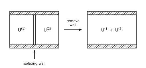
Figure 1 Removing the isolating wall between two subsystems. On the left, a rigid enclosure with hatched top and bottom walls is divided down the middle by a wall drawn as a double line, giving two compartments holding \(U^{\left(1\right)}\) and \(U^{\left(2\right)}\). An arrow labelled “remove wall” leads to the right, where the same enclosure has no divider and holds \(U^{\left(1\right)} + U^{\left(2\right)}\). A short arrow below the first enclosure points up at the divider and labels it the isolating wall.
Subsystems (1) and (2) together are isolated, and the pair relaxes to equilibrium at constant \(U_{\text{total}}\), so \(S\) is maximized:
or
For example, (1) can be filled with gas and (2) is a vacuum. When the wall is removed, the gas expands to fill (1) + (2). Then \(δW_{\text{total}} = 0\) and \(δQ = 0\), so \(ΔU = 0\), but \(ΔS > 0\).
We also postulated that \(S\) is monotonically increasing with \(U\), that is,
Therefore we can always find \(U < U^{\left(1\right)} + U^{\left(2\right)}\) such that
This means that if we let the initial system relax under the constraint of constant \(S\) and \(\vec{x}\), that is, adiabatically reversible, \(U\) will decrease and reach a minimum at equilibrium, or
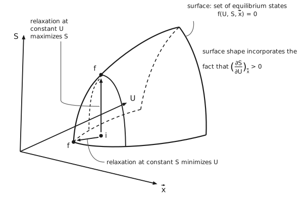
Figure 2 The equilibrium surface. Three solid axes leave a common origin: \(S\) upward, \(\vec{x}\) down to the right, and \(U\) up to the right, into the page. Above them sits a dome shaped like a clothes iron, with a flat base, a nearly vertical back edge on the right, and a front that curves up to a point at the top right. A leader labels the dome’s surface as the surface of equilibrium states, satisfying \(f\left(U, S, \vec{x}\right) = 0\). A second note says that the surface shape incorporates the fact that \(\left(\frac{\partial S}{\partial U}\right)_{\vec{x}} > 0\). Two dashed lines show the dome’s hidden edges: one along the back of the base and one rising nearly vertically to the point, each bowing outward as a mirror image of the solid edge in front of it. Near the front, a cross-section through the starting point \(i\), which sits on the base of the dome, is drawn on the dome as an arch from the top curve down to the base, solid where it is seen and dashed, curving the other way, where it passes behind. Two final states are labelled \(f\), one on the top curve at the top of the arch, directly above \(i\), and one at the vertex where the front of the dome meets the base, below and to the left of \(i\). A solid arrow runs straight up from \(i\) to the first, which is relaxation at constant \(U\), and so maximizes \(S\). A second solid arrow runs down and to the left from \(i\) to the second, which is relaxation at constant \(S\), and so minimizes \(U\). Each arrow carries its own label, with a leader from the label to the arrow.
Imagine that \(i\) comes infinitesimally close to the equilibrium surface. The two final points and \(i\) approach each other, as shown in Figure 2. This represents relaxation from fluctuations away from the equilibrium surface.
Equilibrium criteria for composite systems
Consider \(m\) subsystems with energy \(U^{\left(j\right)}\), entropy \(S^{\left(j\right)}\), and so on. If the total system is isolated and at equilibrium, what is the resulting constraint?
The constraints are
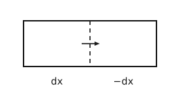
Figure 3 Equal and opposite displacement of an internal partition. A rectangle is divided by a dashed vertical line, and a small arrow pointing to the right crosses the line at its middle. The left part is labelled \(\mathrm{d}x\) and the right part \(- \mathrm{d}x\): a displacement that increases one subsystem decreases the other by the same amount.
subject to
Without loss of generality, take \(m = 2\) as an example:
and, using the constraints (Figure 3),
For any deviations from equilibrium, \(\mathrm{d}U > 0\). At equilibrium, \(\mathrm{d}U = 0\) (Figure 4).
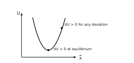
Figure 4 The energy minimum. The vertical axis is \(U\) and the horizontal axis is \(\vec{x}\). A curve dips to a single minimum and rises on both sides. A dot at the minimum is labelled \(\mathrm{d}U = 0\) at equilibrium. A second dot part-way up the rising branch is labelled \(\mathrm{d}U > 0\) for any deviation.
Since \(S^{\left(1\right)}, V^{\left(1\right)}\) and \(N_{i}^{\left(1\right)}\) are independently variable, for \(\mathrm{d}U = 0\) to be true we must have
That is, for a system at equilibrium there can be no gradients in “generalized forces”.
Equilibrium criteria in terms of Legendre transformed variables
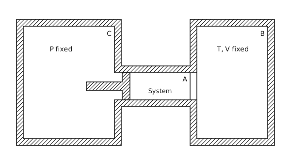
Figure 5 System A between a pressure reservoir and a heat reservoir. A scanned drawing, redrawn here. On the left is a large chamber with hatched walls, labelled \(P\) fixed and lettered C. On the right is a second large chamber with hatched walls, labelled \(T, V\) fixed and lettered B. A channel with hatched walls joins the two at mid-height. In the channel, just inside C, is the piston: a hatched vertical block that spans the channel, with a hatched horizontal rod reaching from it to the left into C, block and rod drawn as one piece. Between the piston and B is a small chamber lettered A and labelled “System”. Its right-hand end, where it meets B, is a wall drawn as two plain lines without hatching. So A exchanges work with C through the piston and heat with B through that wall.
Consider the setup in Figure 5, A + B + C is isolated, and A + B is closed and adiabatic. For both, we have \(\mathrm{d}S_{\text{total}} \le 0\) for deviations away from equilibrium.
First law for A:
Substituting,
which rearranges to the general criterion (for deviations away from equilibrium)
Four cases follow.
\(S\) and \(V\) constant, so \(\mathrm{d}S_{\mathrm{A}} = 0\) and \(δW_{\mathrm{A}} = 0\):
\[\mathrm{d}U_{\mathrm{A}} \ge 0 \implies U \text{ is at a minimum}\]\(S\) and \(P\) constant, so \(\mathrm{d}S_{\mathrm{A}} = 0\) and \(δW_{\mathrm{A}} = - P\mathrm{d}V_{\mathrm{A}}\):
\[- \mathrm{d}\left(U_{\mathrm{A}} + PV_{\mathrm{A}}\right) \le 0 \implies H = U + PV \text{ is at a minimum}\]\(T\) and \(V\) constant, so \(δW_{\mathrm{A}} = 0\):
\[- \mathrm{d}\left(U_{\mathrm{A}} - TS_{\mathrm{A}}\right) \le 0 \implies A = U - TS \text{ is at a minimum}\]\(T\) and \(P\) constant, so \(δW_{\mathrm{A}} = - P\mathrm{d}V_{\mathrm{A}}\):
\[- \mathrm{d}\left(U_{\mathrm{A}} - TS_{\mathrm{A}} + PV_{\mathrm{A}}\right) \le 0 \implies G = U + PV - TS \text{ is at a minimum}\]
Equilibrium for composite systems at fixed temperature and pressure
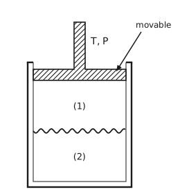
Figure 6 Two phases at fixed temperature and pressure. A vessel is drawn with a doubled wall down its left side, along its bottom and up its right side, with both ends of the doubled wall closed off at the top. The movable piston sits a little way inside the opening between those ends and closes the vessel. The piston is a hatched horizontal slab with a hatched shaft rising from its middle, slab and shaft drawn as one piece. A leader labels the piston “movable”, and the conditions \(T, P\) are marked beside the shaft. A wavy horizontal line across the interior is the phase boundary, with phase (1) above it and phase (2) below.
Closed system constraints:
so that
Notice that we only get the condition of chemical equilibrium from this analysis. This is because \(T\) and \(P\) were fixed across the system at the outset.
Chemical reaction equilibrium
Write the reaction with its stoichiometric coefficients, negative for reactants and positive for products:
Introducing the molar extent of reaction \(ξ\),
Consider a two-phase system at fixed \(T, P\) and initial numbers of moles.
For a closed system,
Substituting,
Since the two variations are independent, both groups vanish separately:
Ideal gas reactions
Substituting into the reaction condition,
The first group is the standard Gibbs free energy of reaction:
and \(K\) is the equilibrium constant:
Phase rule
Derivation
Start from Gibbs-Duhem:
An \(n\)-component, single-phase system has \(n + 1\) intensive variables. An \(n\)-component, \(π\)-phase system therefore has \(π\left(n + 1\right)\) intensive variables, subject to the equalities
Counting them,
which is the number of independently variable intensive properties.
Phase rule and Duhem’s theorem
One component, one phase. Phase rule: \(F = 2\), for example \(T\) and \(p\). Duhem’s theorem: we need to also specify the total number of moles.
One component, two phases. Phase rule: \(F = 1\), for example \(T\) and \(p\). Duhem’s theorem: we need the total number of moles and one more independent extensive property, for example the total volume \(V\).
One component, three phases. Phase rule: \(F = 0\). Duhem’s theorem: we need the total number of moles and two more independent extensive properties, for example the number of moles in two of the three phases.
Two components, three phases. Phase rule: \(F = 1\), for example \(T\). Duhem’s theorem: we need the total number of moles of each species and one more independent extensive variable, for example \(V\).