Homework 1 Solutions
ChE 621 — Thermodynamics.
Problem 1
The variation of the density of water with respect to temperature, at \(P = 1\) atm, can be plotted as follows.
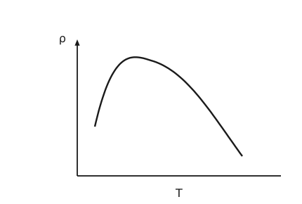
Figure 1 Density of liquid water against temperature at one atmosphere. A sketch with temperature on the horizontal axis and density on the vertical axis, neither carrying numbers. The curve rises from the melting point, \(T = 0\) °C, reaches a maximum at about 4 °C, and then falls again as temperature increases. The maximum is the point of the sketch: a given density below the peak is reached at two different temperatures.
This indicates a maximum in density at a given \(T\), and so there are two \(T\)’s consistent with a given density.
In order to completely characterize the state of pure water, Postulate I requires that we need to specify the mass and two other independently variable properties, that is \(n + 2\) variables.
Let us replot the \(\rho\)–\(T\) projection as a \(\underline{V}\)–\(T\) projection, for a given mass and \(P\).
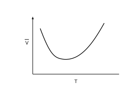
Figure 2 Molar volume against temperature, the same information inverted. A sketch with temperature on the horizontal axis and molar volume on the vertical axis, neither carrying numbers. The curve decreases from the melting point, \(T = 0\) °C, reaches a minimum at about 4 °C, and then rises again as temperature increases. The minimum sits at the same temperature as the maximum of Figure 1, since the molar volume is inversely proportional to the density.
Now, we are in the one-phase liquid region of the phase diagram, so \(P\) and \(T\) are independently variable, as are the other pairs \(P\), \(\underline{V}\) and \(T\), \(\underline{V}\).
Are we at liberty to specify any one of these three pairs to determine uniquely all other properties of the system?
The pair \(P\), \(\underline{V}\)
If one specifies \(P = 1\) atm and \(\underline{V}\), the previous plot reveals that there are two temperatures consistent with the same \(P\), \(\underline{V}\) choice. This contradicts Postulates I and II, since the system has reached a unique stable equilibrium state, but cannot be completely characterized by the mass and the two independently variable properties \(P\) and \(\underline{V}\), a total of \(n + 2\) variables, as required by Postulate I. \(P\), \(\underline{V}\), and the mass yield two \(T\)’s, and we apparently need more information in order to distinguish between the two equilibrium states of water. To ensure that the system approaches a unique stable equilibrium state, we appear to need more variables than just \(n + 2\), but which ones?
The pair \(T\), \(\underline{V}\)
Each \(T\), \(\underline{V}\) pair, and the mass, yields only one value for \(P\). Hence Postulates I and II are satisfied, that is, only \(n + 2\) variables are needed to describe the unique stable equilibrium state.
The pair \(P\), \(T\)
Each \(P\), \(T\) pair, and the mass, yields only one value for \(\underline{V}\). Thus Postulates I and II are also satisfied.
Why the first pair fails
Although \(P\) and \(\underline{V}\) are independently variable in the one-phase region, and we can certainly vary \(\underline{V}\) while keeping \(P\) constant and the other way round while staying in the one-phase region, why does this pair fail to satisfy Postulates I and II? What sets it apart from \(T\), \(\underline{V}\) and \(T\), \(P\)?
\(P\) and \(\underline{V}\) are conjugate variables. There are certain instances, the density maximum of water being one example, in which conjugate pairs fail to specify completely the given system.
Thus Postulate I should be modified to read: “characterized completely by two independently variable non-conjugate properties in addition to the masses…”
Problem 2
Take the oxide as the system.
with
Problem 3
Consider the state function \(PV\), whose differential can be written as
The left-hand side is exact. The two terms on the right are inexact.
Let us now integrate each of the above two inexact differentials along the given arbitrary path beginning at \(P_{1}, V_{1}\) and ending at \(P_{2}, V_{2}\). The integral over \(P\,\mathrm{d}V\) simply yields the area below the curve, where for the direction of the given pathway \(\mathrm{d}V > 0\).
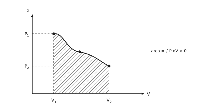
Figure 3 The integral of \(P\,\mathrm{d}V\) as the area under the path. A pressure-volume diagram. Pressure is on the vertical axis, volume on the horizontal. An arbitrary path runs from a filled point at \(P_{1}, V_{1}\) at the upper left, wanders downward and to the right with a slight shelf in the middle, and ends at a filled point at \(P_{2}, V_{2}\) at the lower right. An arrowhead partway along shows the direction of travel. Dashed guide lines drop from each end point to the axes and mark \(P_{1}\), \(P_{2}\), \(V_{1}\) and \(V_{2}\). The region bounded above by the path, below by the volume axis, and on the sides by \(V_{1}\) and \(V_{2}\) is hatched. It is labelled: area = the integral of \(P\,\mathrm{d}V\), which is greater than zero.
Now, the integral over \(V\,\mathrm{d}P\) yields the area to the left of the curve, shown in Figure 4. Note that for the direction of the given pathway, for which \(\mathrm{d}P < 0\), we have \(V\,\mathrm{d}P < 0\).
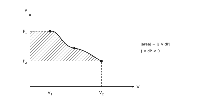
Figure 4 The integral of \(V\,\mathrm{d}P\) as the area to the left of the path. The same pressure-volume diagram and the same path. This time the hatched region is bounded on the right by the path, on the left by the pressure axis, and above and below by \(P_{1}\) and \(P_{2}\). It is labelled: the magnitude of the area equals the magnitude of the integral of \(V\,\mathrm{d}P\), and the integral of \(V\,\mathrm{d}P\) is less than zero.
So the sum of the two areas, one positive and one negative, yields the following in Figure 5.
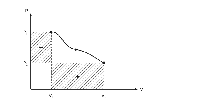
Figure 5 The sum of the two areas. The same path again, with two hatched rectangles instead of the curved regions. The first spans from the pressure axis out to \(V_{1}\), and from \(P_{2}\) up to \(P_{1}\), and is marked with a minus sign. The second spans from \(V_{1}\) to \(V_{2}\), and from the volume axis up to \(P_{2}\), and is marked with a plus sign. The area inside the shape bounded by the curve itself has cancelled between the two integrals and is not shaded.
Note that the area inside the “triangle”, or the area bounded by the given curve and the lines \(P_{1}, V_{1}\) to \(P_{2}, V_{1}\) and \(P_{2}, V_{1}\) to \(P_{2}, V_{2}\), cancels, or yields a zero net contribution to the sum.
So the final result, regardless of the path taken between \(P_{1}, V_{1}\) and \(P_{2}, V_{2}\), is always equal to the sum of the areas of the two rectangles, one positive and one negative, in the above figure:
where the first term is greater than zero and the second is less than zero, so that
So, while \(\int P\,\mathrm{d}V\) and \(\int V\,\mathrm{d}P\) are both path dependent, their sum is path-independent, \(\int \mathrm{d}(PV)\).
Note that the above graphical analysis is still valid even if the given pathway rises above \(P_{1}\) or extends beyond \(V_{2}\).
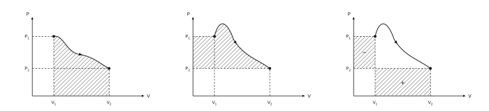
Figure 6 The same construction when the path leaves the rectangle. Three small pressure-volume diagrams side by side. In each, the path climbs above \(P_{1}\) shortly after leaving \(P_{1}, V_{1}\) before falling to \(P_{2}, V_{2}\). The first has the area under the path hatched, the second the area to the left of it, and the third the same two rectangles as Figure 5, again marked minus and plus. The rectangles are unchanged by the excursion, which is the point: the construction does not depend on the path staying inside them.
Problem 4
Part a
The above implies that
Now
Since these mixed second-order partial derivatives are equal, \(\mathrm{d}w\) is an exact differential. Hence some analytic function \(w(x, y)\) exists whose differential is given by the above expression for \(\mathrm{d}w\).
Since \(\mathrm{d}w\) is an exact differential, the integral of \(\mathrm{d}w\) between the same two end points will be independent of the path taken. So, integrate \(\mathrm{d}w\) from some initial point \(x_{0}, y_{0}\) to the final point \(x, y\) over the following, and convenient, path: go from \(x_{0}\) to \(x\) at constant \(y_{0}\), and then from \(y_{0}\) to \(y\) at constant \(x\).
Step 1.
Step 2.
So
Since \(y_{0}\), \(x_{0}\) and \(w(x_{0}, y_{0})\) are arbitrary constants, \(w(x_{0}, y_{0})\) being simply a constant of integration, the most general form of \(w\) is
The total differential of the above function is, as expected, given by
Part b
The above implies that
Now,
Since these mixed second-order partial derivatives are unequal, \(\mathrm{d}w\) is an inexact differential. Hence there is no analytic function of \(x\) and \(y\) that would yield the above total differential. We do know, however, that every Pfaff differential expression in two dimensions possesses an integrating factor, or denominator, which when multiplying, or dividing, the inexact differential renders it exact. In other words, there is some function \(\mu = \mu(x, y)\) such that
Now,
where \(\mu_{x}\) and \(\mu_{y}\) represent the first partial derivatives of \(\mu\) with respect to \(x\) and \(y\) respectively. If \(\mathrm{d}w\) is exact, the above mixed second-order partial derivatives must be equal. Therefore,
Let us assume that \(\mu\) can be represented by the product of two separate functions, \(\mu = g(x)h(y)\), which when substituted into the above partial differential equation yields
The left-hand side is only a function of \(y\), while the right-hand side is only a function of \(x\). Both must therefore be equal to the same constant \(k\). The solutions of the two separate first-order ordinary differential equations are
where \(c_{1}\) and \(c_{2}\) are constants. Finally, we note that
And so the integrating denominator is
Substitution of the above integrating denominator into the original inexact differential yields
which is now an exact differential. Note that we have in fact found an infinite number of integrating denominators, all dependent upon the choice of \(k\) and \(A\). The function corresponding to the above differential is simply
Part c
Note that
Since these two derivatives are unequal, \(\mathrm{d}F\) is an inexact differential. Hence there is no analytic function of \(x\), \(y\) and \(z\) that would yield the above total differential.
Part d
Now,
Hence \(\mathrm{d}U\) is an exact differential. To find \(U\), integrate along the following convenient path: \(x_{0}\) to \(x\) at \(y_{0}, z_{0}\); then \(y_{0}\) to \(y\) at \(x, z_{0}\); then \(z_{0}\) to \(z\) at \(x, y\). So
or
Problem 5
Throughout, gas A and gas B are the same diatomic ideal gas with \(\tilde{C}_{V} = \tfrac{5}{2}R\), the cylinder is 0.5 m long, and initially \(V_{A0} = 2V_{B0}\), \(T_{A0} = T_{B0} = T_{0} = 300\) K, \(P_{A0} = 10\) bar and \(P_{B0} = 1\) bar.
Part a: no reservoir, diathermal piston
Since the piston is diathermal, the final temperature of gas A and gas B should be the same, \(T_{A1} = T_{B1} = T_{1}\). And we also have \(P_{A1} = P_{B1} = P_{1}\). So
and
so that
Apply the first law for the A plus B system:
Part b: no reservoir, adiabatic piston
Let \(V_{A0} = \tfrac{2}{3}V_{0}\) and \(V_{B0} = \tfrac{1}{3}V_{0}\). Apply the first law for A plus B:
If we assume all the friction heat goes back entirely to A, then B undergoes a reversible, adiabatic pathway.
Also, \(n_{A}RT_{A1} = P_{A1}V_{A1}\) and \(n_{B}RT_{B1} = P_{B1}V_{B1}\) with \(P_{A1} = P_{B1} = P_{1}\), so
And
Solving Equation (1), Equation (2), Equation (3) and Equation (4) yields
If instead we assume all the friction returns back entirely to B as heat, then A undergoes a reversible, adiabatic pathway. So
Solving Equation (1), Equation (5), Equation (3) and Equation (4) simultaneously gives
So, on average,
Part c: reservoir, diathermal piston
Part d: reservoir, adiabatic piston
Assume all the friction returns to A, so that B follows an adiabatic pathway. Then
Solving Equation (6), Equation (7) and Equation (8), we get
Assume instead that all the friction returns to B, so that A follows an isothermal process. Apply the first law on gas A plus B, with \(\mathrm{d}U_{A} = 0\) and \(W = 0\):
Apply the first law on A, for which \(\mathrm{d}U_{A} = Q + W_{A} = 0\), so that
Solving Equation (7), Equation (8) and Equation (9) gives
On average,
Part d, worked the other way: isothermal reversible expansion in A
Alternatively, if we assume isothermal reversible expansion in A:
If we take A plus B as the system, then \(\mathrm{d}U_{A} + \mathrm{d}U_{B} = \delta Q + \delta W\), in which \(\mathrm{d}U_{A} = 0\) because A is isothermal and \(\delta W = 0\).
If we take A as the system, then \(\mathrm{d}U_{A} = \delta Q_{A} + \delta W = 0\).
We also have \(\delta Q = \delta Q_{A}\), as only A is in contact with the heat reservoir. Therefore
At equilibrium, \(n_{A}RT_{A} = P_{A}V_{A}\) and \(n_{B}RT_{B} = P_{B}V_{B}\), so that
Note how different these answers are depending on our assumptions about the path. For parts b and d, since A is at a higher pressure and expands against B, it appears more reasonable to assume B is adiabatic and reversible.