Thermodynamics of Mixtures
ChE 621 — Thermodynamics.
Concept of partial molar properties
For an extensive property \(M\), which may be \(V, H, G\) and so on, the partial molar property of species \(i\) is
For example, with \(M = G\),
is the chemical potential.
Physical interpretation
What is the volume change when one drop of B is added to a mixture of A and B (Figure 1)?
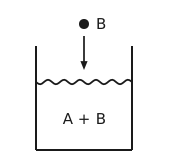
Figure 1 Adding a drop of B to a mixture. An open vessel holding a liquid labelled A + B, its surface drawn wavy. A small drop labelled B hangs above it, with an arrow pointing down from the drop to the surface.
In general the molar volume of pure B does not do the job:
but we can always write
and define the partial molar volume as the limit of that effective molar volume,
For a pure species the two coincide: \(\bar{V}_{\mathrm{B}} = \tilde{V}_{\mathrm{B}}\).
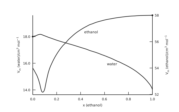
Figure 2 Partial molar volumes in the water-ethanol system. The horizontal axis is the mole fraction of ethanol from 0.0 to 1.0. The left vertical axis is the partial molar volume of water in cubic centimetres per mole, ticked at 14.0, 16.0 and 18.0; the right vertical axis is the partial molar volume of ethanol on the same kind of scale, ticked at 52, 54, 56 and 58. The curve labelled water starts from a marked point at exactly 18.0 in pure water, rises very slightly to a shallow maximum near a mole fraction of 0.06, then falls away, gently at first and steeply at the far right, ending near 14.0 in pure ethanol. The curve labelled ethanol starts near 54.0, drops to a sharp minimum of about 52.2 near a mole fraction of 0.085, then climbs steeply, flattens out across the middle of the diagram and reaches a marked point at exactly 58 in pure ethanol. The two curves cross near a mole fraction of 0.27. Each curve therefore meets the pure-component molar volume at its own end of the diagram, and departs from it everywhere else.
Identities of partial molar properties
Consider any extensive property \(M\), which may be \(G, V, H\) and so on, of a mixture of \(N\) species with mole numbers \(n_{1}, n_{2}, \dots, n_{N}\), and let
Then
Let \(x_{i} = \frac{n_{i}}{n}\), so that \(\mathrm{d}n_{i} = n \mathrm{d}x_{i} + x_{i} \mathrm{d}n\). Also \(M = n \tilde{M}\), so
Equating the two expressions and collecting terms gives
Both brackets must vanish separately, because \(n\) and \(\mathrm{d}n\) are independent.
Second bracket:
First bracket:
which leaves the Gibbs-Duhem equation:
With \(M = G\), so that \(\bar{M}_{i} = μ_{i}\),
and therefore
Calculation of partial molar quantities from experimental data
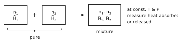
Figure 3 Measuring an enthalpy of mixing. Two boxes side by side, joined by a plus sign: the first holds \(n_{1}\) moles of pure species 1 with molar enthalpy \(\tilde{H}_{1}\), the second \(n_{2}\) moles of pure species 2 with molar enthalpy \(\tilde{H}_{2}\). A brace under the two boxes labels them pure. An arrow leads from them to a third, larger box labelled mixture, holding both species together, whose enthalpies are now the partial molar values \(\bar{H}_{1}\) and \(\bar{H}_{2}\). Written beside the sketch: at const. \(T\) & \(P\), measure heat absorbed or released.
Consider a binary mixture made from mixing two pure components, shown in Figure 3. The enthalpy of mixing is the difference between the mixture and the pure components:
Dividing by \(n = n_{1} + n_{2}\),
On a plot of \(Δ\tilde{H}_{\text{mixing}}\) against \(x_{2}\) (Figure 4), the slope can be found by differentiating with respect to \(x_{2}\),
The last two terms sum to zero by the Gibbs-Duhem equation. We can find the tangent line
by matching \(y\left(x_{2}\right)\) with \(Δ\tilde{H}_{\text{mixing}\left(x_{2}\right)}\):
and therefore the intercept gives (Figure 4)
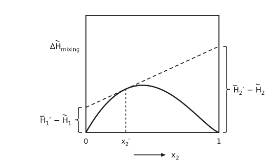
Figure 4 The tangent construction on the enthalpy of mixing. \(Δ\tilde{H}_{\text{mixing}}\) against \(x_{2}\) in a closed frame, from 0 to 1, both ends of the curve pinned at zero since a pure component has no enthalpy of mixing. The curve rises steeply from 0, peaks a little left of the middle and falls back to zero at 1, flattening as it arrives. A dashed straight line touches the curve at a composition \(x_{2}'\) on the rising side, left of the peak, marked by a dashed vertical down to the axis. The line is extended to both edges of the frame, so it rises from left to right and ends above the peak of the curve. A brace at the left edge spans the intercept there and points left to its label, \(\bar{H}_{1}' - \tilde{H}_{1}\), and a brace at the right edge spans the intercept there and points right to its label, \(\bar{H}_{2}' - \tilde{H}_{2}\). The construction is the point of the algebra that follows: the tangent at one composition reads off both partial molar enthalpies at that composition.
Ideal gas mixture

Figure 5 Mixing pure ideal gases. A row of boxes joined by plus signs, each holding one pure species: the first \(n_{1}\) moles at pressure \(P_{1}\) with chemical potential \(μ_{1}\) and entropy \(S_{1}\), the second \(n_{2}\) moles at \(P_{2}\) with \(μ_{2}\) and \(S_{2}\), and so on. An arrow leads to a single box holding the mixture at total pressure \(P\) with \(n\) moles, and with a chemical potential, enthalpy and entropy of its own.
The ideal-gase equation of state
assumes 1) non-interacting molecules with 2) zero volume. Mixing ideal gases (Figure 5) should preserve both assumptions. Let the mole fraction
We can define the partial pressure
Gibbs theorem: a partial molar property, except \(V\), of a constituent species in an ideal gas mixture is equal to the corresponding molar property of the species as a pure ideal gas at the mixture temperature but at a pressure equal to its partial pressure in the mixture:
Example 1, enthalpy.
\(H\) does not depend on \(P\), so \(\bar{H}^{\text{ig}} = \tilde{H}^{\text{ig}}\), and therefore
Example 2, entropy.
so that \(\mathrm{d}\tilde{S}^{\text{ig}} = - R \, \mathrm{d}\ln P\) at constant \(T\), and
Chemical potential of species \(i\) in an ideal gas mixture
so
Differentiating the Gibbs energy of mixing with respect to pressure gives the volume of mixing:
so that \(\bar{V}_{i}\) at \(\left(T, P\right)\) equals \(\tilde{V}_{i}\) at \(\left(T, P\right)\), not at \(\left(T, P_{i}\right)\). The partial molar volume is the exception in Gibbs’ theorem.
Ideal solutions (mixtures)
By analogy to the ideal gas, where
If we group the first two terms as \(μ_{i}^{*}\left(T, P\right)\),
Mixtures satisfying this equation are called ideal solutions. The first term is the pure-component chemical potential \(\tilde{G}_{i}\left(T, P\right)\), and for solids and liquids it may not be \(\tilde{G}_{i}^{\circ}\left(T\right) + RT \ln P\).
Mixtures behave like ideal solutions at high pressure, as gases, liquids and solids. It is possible to have an “ideal mixture of non-ideal gases” (i.e., for which \(P\tilde{V} \ne RT\)).
Differentiating with respect to pressure,
\[\left(\frac{\partial μ_{i}}{\partial P}\right)_{T,\, n_{i}} = \left(\frac{\partial μ_{i}^{*}}{\partial P}\right)_{T,\, n_{i}}\]
so that
Similarly,
The three ideal-solution properties are therefore
Note that (Figure 6)
The ideal-solution model works well when 1) the species are not different in size and 2) their chemical interactions are similar. Examples: \(n\)-heptane with \(n\)-hexane, ethanol with propanol, silicon with germanium, zinc with copper.
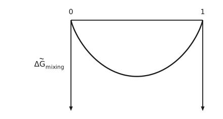
Figure 6 The ideal Gibbs energy of mixing. \(Δ\tilde{G}_{\text{mixing}}\) plotted downward from a horizontal zero line whose ends are marked 0 and 1. A vertical axis drops from each end of the line, its arrow pointing down, the direction in which \(Δ\tilde{G}_{\text{mixing}}\) grows more negative. The curve leaves zero steeply at both ends and dips symmetrically below in between, reaching its most negative value at equal composition. The whole curve lies below zero, which is the point: ideal mixing always lowers the Gibbs energy, so an ideal mixture never separates.
Ideal vapor-liquid phase equilibrium
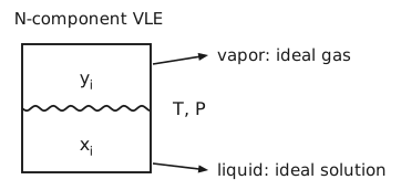
Figure 7 The \(N\)-component vapor-liquid equilibrium. A closed vessel divided by a wavy interface, under the heading \(N\)-component VLE. The upper region is labelled with the vapor mole fractions \(y_{i}\) and the lower with the liquid mole fractions \(x_{i}\), and the vessel is marked \(T, P\) beside it. Two arrows lead out of the right side of the vessel to labels: vapor: ideal gas, from the upper region, and liquid: ideal solution, from the lower.
If the vapor and liquid phases are assumed to be ideal gas and ideal solution, respectively (Figure 7), writing each side with its own reference,
For the vapor, \(\frac{\partial \tilde{G}^{\text{ig}}}{\partial P} = \tilde{V}^{\text{ig}}\), so
For the liquid, \(\frac{\partial \tilde{G}_{i}^{\mathrm{L}}}{\partial P} = \tilde{V}^{\mathrm{L}}\), which is small, so
Equation (1) then becomes
Therefore \(RT \ln \frac{P y_{i}}{P_{i}^{\text{sat}}} = RT \ln x_{i}\), which is Raoult’s law:
For a binary mixture the total pressure is linear in the liquid composition (Figure 8):
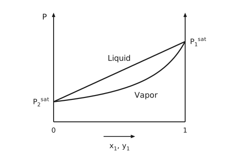
Figure 8 Pressure against composition at fixed temperature. The vertical axis is pressure, the horizontal axis runs from 0 to 1 in \(x_{1}\) and \(y_{1}\). Two curves join the pure-component saturation pressures, \(P_{2}^{\text{sat}}\) at the left edge and the higher \(P_{1}^{\text{sat}}\) at the right edge. The upper of the two, the bubble line, is a straight line, because the total pressure of an ideal solution is linear in liquid composition. The lower, the dew line, sags below it, because the vapor composition is not the liquid composition. The region above both curves is labelled Liquid, the region below them Vapor, and the lens between them is the two-phase region. Both vertical sides carry arrows, and the frame is open at the top.
Ideal liquid-solid phase diagrams
To draw a \(T\)-\(x\) diagram we need \(x_{i}^{\mathrm{S}}\) and \(x_{i}^{\mathrm{L}}\) as functions of \(T\). Equating chemical potentials in the two phases,
Differentiating with respect to temperature,
and integrating,
For a binary system A-B this is one equation per species:
A mass balance on species A over the two phases,
gives the lever rule (Figure 9):
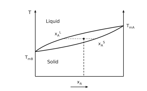
Figure 9 A liquid-solid temperature-composition diagram. Temperature on the vertical axis against \(x_{\mathrm{A}}\), with an arrow on each vertical side and the frame open at the top. Two curves, computed for ideal solid and liquid solutions, run from the melting temperature of pure B, \(T_{\text{mB}}\) on the left axis, to that of pure A, \(T_{\text{mA}}\), at the right edge, opening into a lens between them. The upper curve is the liquidus and the lower the solidus. The region above the lens is labelled Liquid and the region below it Solid. A dotted horizontal tie line at one temperature runs across the lens from the liquidus at \(x_{\mathrm{A}}^{\mathrm{L}}\) to the solidus at \(x_{\mathrm{A}}^{\mathrm{S}}\), the compositions of the coexisting phases. A dot on the tie line marks one overall composition, and a dashed vertical line runs from it down to the composition axis. The lever rule that follows divides the tie line at that point.
Freezing point depression (liquid-solid)
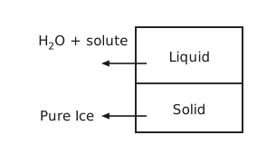
Figure 10 Ice in equilibrium with a solution. A closed vessel divided by a horizontal interface. The upper region is labelled Liquid, and an arrow from it points out to the label H\(_{2}\)O + solute. The lower region is labelled Solid, and an arrow from it points out to the label Pure Ice. The solute enters only the liquid, which is why there is only the chemical potential equality for the solvent.
For a solvent in equilibrium with its own pure solid (Figure 10),
where \(Δ\tilde{H}_{i}^{\text{SL}}\) is the latent heat of melting for pure \(i\). Inverting,
The derivative is positive in \(x_{\text{solv.}}\), and since \(x_{\text{solute}} = 1 - x_{\text{solv.}}\) so that \(\mathrm{d}x_{\text{solute}} = - \mathrm{d}x_{\text{solv.}}\), the melting temperature falls as solute is added (Figure 11).
To get the exact \(x\) dependence of \(T_{\mathrm{m}}\), integrate
which needs the temperature dependence of \(Δ\tilde{H}_{i}^{\text{SL}}\):
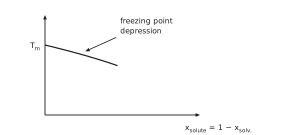
Figure 11 Freezing point depression. Temperature on the vertical axis against the solute mole fraction \(x_{\text{solute}} = 1 - x_{\text{solv.}}\) on the horizontal. The vertical axis is marked only at \(T_{\mathrm{m}}\), the melting temperature of the pure solvent, where the curve starts. The curve, computed for an ideal solution, falls almost linearly across the first half of the axis as solute is added. An arrow from the label freezing point depression points at the curve. The sign is the content of the figure: adding solute lowers the temperature at which the solid appears.
Boiling point elevation (liquid-vapor)
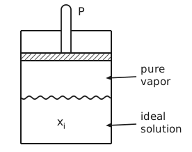
Figure 12 Boiling an ideal solution at fixed pressure. A cylinder closed at the top, with a rod through the top to a hatched piston, the rod labelled \(P\). Between the piston and a wavy liquid surface is pure vapor, and below the surface the ideal solution of composition \(x_{i}\). Labels to the right, pure vapor and ideal solution, have arrows pointing into the two regions. The solute is non-volatile, so only the solvent is in the vapor.
Consider a non-volatile solute dissolved in a solvent (Figure 12):
where \(Δ\tilde{H}^{\text{LV}}\) is the latent heat of vaporization, and therefore
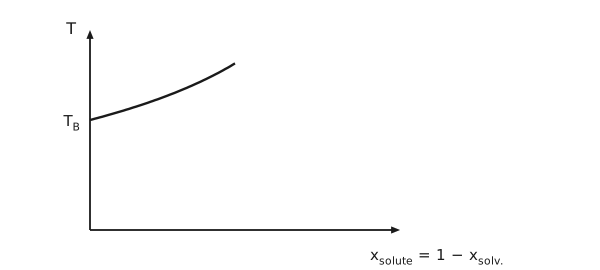
Figure 13 Boiling point elevation. Temperature on the vertical axis, labelled \(T\), against the solute mole fraction \(x_{\text{solute}} = 1 - x_{\text{solv.}}\) on the horizontal. The curve starts at the boiling temperature of the pure solvent, marked \(T_{\mathrm{B}}\) on the vertical axis, and, computed for an ideal solution, rises steadily across the first half of the axis as solute is added. The sign is opposite to that of the previous pair of figures: adding solute raises the temperature at which the liquid boils.
Osmotic pressure
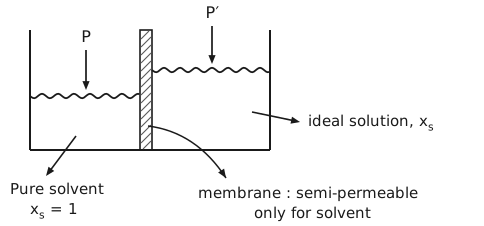
Figure 14 An osmotic cell. A vessel open at the top, split into two chambers by a hatched vertical membrane. The left chamber holds pure solvent, labelled Pure solvent, \(x_{\mathrm{s}} = 1\), and an arrow labelled \(P\) presses on its wavy surface. The right chamber holds the ideal solution, labelled ideal solution, \(x_{\mathrm{s}}\). Its surface stands higher, and an arrow labelled \(P'\) presses on it. A curved arrow from the membrane leads to its label, membrane: semi-permeable, only for solvent, which is what makes the two pressures different at equilibrium.
Consider a semi-permeable membrane that only allows solvent molecules to pass through (Figure 14). Solvent will flow into the solution because its chemical potential is lower there, an entropic driving force, until a sufficient pressure difference develops. At equilibrium the solvent has the same chemical potential on both sides:
Denoting the osmotic pressure \(Π = P' - P\), and using \(\left(\frac{\partial μ_{\mathrm{s}}^{*}}{\partial P}\right)_{T} = \tilde{V}_{\mathrm{s}}\),
assuming \(\tilde{V}_{\mathrm{s}}\) is constant over a not too large pressure range. Therefore
Ideal dilute solutions
For an ideal solution, both
hold over the complete concentration range, as a direct consequence of \(μ_{i} = μ_{i}^{*}\left(T, P\right) + RT \ln x_{i}\).
Now take \(i = \mathrm{CO}_{2}\) in H\(_{2}\)O at low concentrations. The pure-liquid reference \(μ_{\mathrm{CO}_{2}}^{*}\left(T, P\right)\) does not even exist, but \(μ_{\mathrm{CO}_{2}}\) still changes with \(RT \ln x_{i}\), so we can write
This leads to the ideal dilute solution (Figure 15 – Figure 17). For the dilute solute, \(x_{i} \to 0\),
For the solvent, \(x_{i} \to 1\), the ideal solution applies,
At each end of the composition range, one species follows the ideal solution and the other the ideal dilute solution:
as \(x_{2} \to 0\) and \(x_{1} \to 1\), species 2 follows the ideal dilute solution, \(μ_{2} = μ_{2}^{\infty} + RT \ln x_{2}\), and species 1 the ideal solution, \(μ_{1} = μ_{1}^{*} + RT \ln x_{1}\);
as \(x_{2} \to 1\) and \(x_{1} \to 0\), species 2 follows the ideal solution, \(μ_{2} = μ_{2}^{*} + RT \ln x_{2}\), and species 1 the ideal dilute solution, \(μ_{1} = μ_{1}^{\infty} + RT \ln x_{1}\).
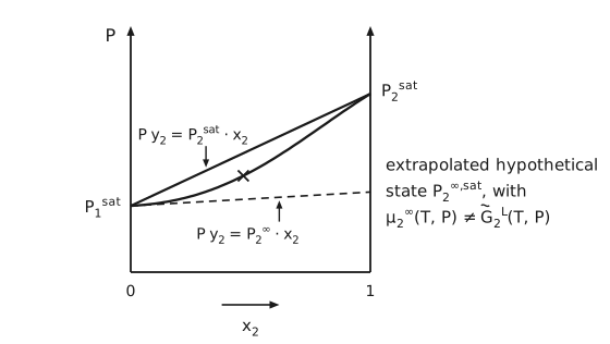
Figure 15 The ideal-solution line and the extrapolated hypothetical state. Pressure \(P\) against \(x_{2}\), from 0 to 1, with an arrow on each vertical side. \(P_{1}^{\text{sat}}\) is marked low on the left axis and \(P_{2}^{\text{sat}}\) higher on the right. A straight line joins them, labelled \(P y_{2} = P_{2}^{\text{sat}} \cdot x_{2}\) by an arrow from above. Below it a curve, computed for a mixture with a negative deviation from Raoult’s law, also joins the two: it leaves \(P_{1}^{\text{sat}}\) almost flat, rises through a point marked with a cross, and meets the straight line at \(P_{2}^{\text{sat}}\). A dashed line, the tangent to the curve at \(P_{1}^{\text{sat}}\), the infinite-dilution limit, runs from there across to the right axis, where it ends below \(P_{2}^{\text{sat}}\), and an arrow from below labels it \(P y_{2} = P_{2}^{\infty} \cdot x_{2}\). The note beside the plot reads: extrapolated hypothetical state \(P_{2}^{\infty,\text{sat}}\), with \(μ_{2}^{\infty}\left(T, P\right) \ne \tilde{G}_{2}^{\mathrm{L}}\left(T, P\right)\).
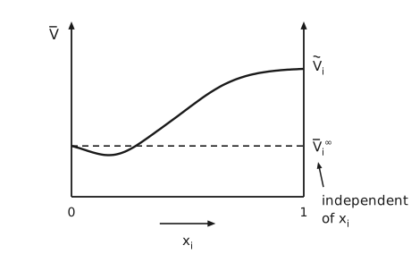
Figure 16 The partial molar volume near infinite dilution. \(\bar{V}\) on the vertical axis against \(x_{i}\) on the horizontal, from 0 to 1, with an arrow on each vertical side. The curve begins at a finite value on the left axis, dips slightly, then rises and levels off at the pure-component molar volume \(\tilde{V}_{i}\) on the right axis. A dashed horizontal line runs from the starting value to the right axis, labelled \(\bar{V}_{i}^{\infty}\), and an arrow from the note independent of \(x_{i}\) points up at that label. The partial molar volume at infinite dilution is therefore a well-defined property of the solute in that solvent even though the pure solute may not exist as a liquid at all.
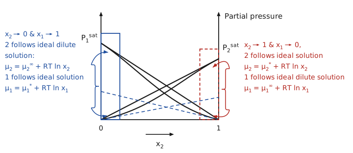
Figure 17 Both ends of a binary partial-pressure diagram. Partial pressure against \(x_{2}\), from 0 to 1, with an arrow on each vertical side. Species 1 falls from \(P_{1}^{\text{sat}}\) on the left axis to zero at the right, and species 2 rises from zero at the left to the lower \(P_{2}^{\text{sat}}\) on the right axis. Each species has a straight line, its Raoult’s law line \(P_{i} = P_{i}^{\text{sat}} x_{i}\), and a curve that sags below it, computed for a mixture with a negative deviation from Raoult’s law. Each curve runs along its straight line where that species is nearly pure. Where the species is dilute, the curve runs along a dashed blue line instead, its Henry’s law line, which ends on the far axis below the saturation pressure. A solid blue box encloses the end near \(x_{2} = 0\) and a dashed red box the end near \(x_{2} = 1\). A blue brace on the left, with one arrow to the top of the blue box and one to its foot, carries the note: \(x_{2} \to 0\) and \(x_{1} \to 1\), 2 follows ideal dilute solution, \(μ_{2} = μ_{2}^{\infty} + RT \ln x_{2}\), 1 follows ideal solution, \(μ_{1} = μ_{1}^{*} + RT \ln x_{1}\). A red brace on the right, with arrows into the red box, carries the note: \(x_{2} \to 1\) and \(x_{1} \to 0\), 2 follows ideal solution, \(μ_{2} = μ_{2}^{*} + RT \ln x_{2}\), 1 follows ideal dilute solution, \(μ_{1} = μ_{1}^{\infty} + RT \ln x_{1}\).
Phase equilibrium in dilute solutions of gases
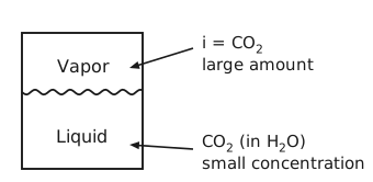
Figure 18 A gas dissolved in a liquid. A closed vessel divided by a wavy interface, the upper region labelled Vapor and the lower Liquid. Labels to the right point into the two regions with arrows: \(i = \mathrm{CO}_{2}\), large amount, into the vapor, and CO\(_{2}\) (in H\(_{2}\)O), small concentration, into the liquid. The asymmetry is the point: the same species is nearly pure in one phase and dilute in the other, so the two phases need different references.
As shown in Figure 18,
Rearranging,
Ideal liquid-liquid equilibrium
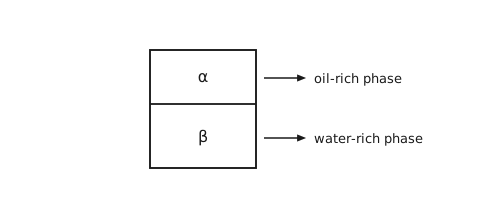
Figure 19 Two immiscible liquid phases. A vessel divided by a horizontal interface into an upper phase labelled \(α\), the oil-rich phase, and a lower phase labelled \(β\), the water-rich phase. The two phases are immiscible and therefore non-ideal, since an ideal mixture always has a negative Gibbs energy of mixing and so never separates.
Consider a third, dilute component distributed between two immiscible liquid phases (Figure 19), \(μ_{i}^{\left(α\right)} = μ_{i}^{\left(β\right)}\).
The two phases \(α\) and \(β\) are immiscible and therefore non-ideal, since ideal mixtures always have