Second Law of Thermodynamics
ChE 621 — Thermodynamics.
Heat engines and statements of the second law
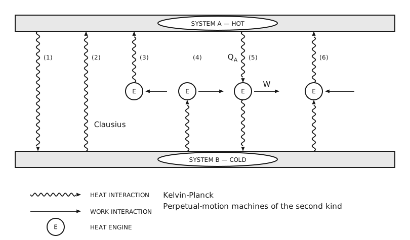
Figure 1 Conceivable heat and work interactions between a hot system and a cold system. A wide horizontal bar across the top is labelled “system A — hot” and a matching bar across the bottom is labelled “system B — cold”. Six interactions are numbered from left to right in the space between them. In (1) a wavy line runs from A down to B, so heat passes from the hot system to the cold one. In (2) a wavy line runs from B up to A, so heat passes from the cold system to the hot one with nothing else happening. In (3) a heat engine sits just below A: a straight arrow carries work into the engine from the right, and a wavy line carries heat from the engine up into A. In (4) a heat engine sits just above B: a wavy line carries heat from B up into the engine, and a straight arrow carries work out of the engine to the right. In (5) a heat engine sits between the two: a wavy line labelled \(Q_{A}\) carries heat from A down into it, a straight arrow labelled \(W\) carries work out to the right, and a wavy line carries the remaining heat down into B. In (6) a heat engine again sits between the two, but the directions are reversed: a wavy line carries heat from B up into the engine, a straight arrow carries work into the engine from the right, and a wavy line carries heat from the engine up into A. The typed word “Clausius” stands beside interaction (2), naming the transfer that the Clausius statement forbids. Below the cold bar, and to the right of interaction (4), the typed lines “Kelvin-Planck” and “Perpetual-motion machines of the second kind” name what the right-hand group of interactions would be. A legend gives the three symbols: a wavy line with an arrowhead is a heat interaction, a straight line with an arrowhead is a work interaction, and a circle lettered E is a heat engine.
With the convention \(θ_{A} > θ_{B}\), so that
the efficiency of the engine of interaction (5) is
Clausius statement of the second law of thermodynamics
Heat cannot pass spontaneously from a body at a lower temperature to a body at a higher temperature.
Kelvin/Planck statement of the second law of thermodynamics
Any cyclic process in which the net effect is the transfer of energy from a single system and conversion of that energy into work is impossible.
The efficiency must be a function of both temperatures
\(η\) must be a function of both \(θ_{A}\) and \(θ_{B}\).
Prove this by assuming instead that
and using the construct in Figure 2.
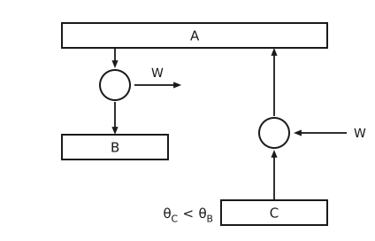
Figure 2 Construct used to rule out an efficiency that depends on one temperature alone. A bar labelled A runs across the top. Below it on the left, an arrow carries heat down from A into a circular engine, a horizontal arrow labelled \(W\) carries work out of that engine to the right, and a further arrow carries heat down from the engine into a bar labelled \(B\). On the right, a second circular engine is driven backwards: an arrow labelled \(W\) carries work into it from the right, an arrow carries heat up into it from a bar labelled \(C\) at the bottom, and an arrow carries heat from it up into A. To the left of the \(C\) bar, and below the \(B\) bar, is the condition \(θ_{C} < θ_{B}\).
Therefore, we have
What form must the efficiency satisfy?
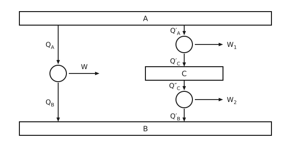
Figure 3 A single engine between A and \(B\) compared with two engines in series through \(C\). A bar labelled A runs across the top and a bar labelled \(B\) across the bottom, with a shorter bar labelled \(C\) in the middle of the right-hand side. On the left, one engine takes heat \(Q_{A}\) down from A, delivers work \(W\) to the right, and rejects heat \(Q_{B}\) down to \(B\). On the right, an upper engine takes heat \(Q'_{A}\) down from A, delivers work \(W_{1}\) to the right, and rejects heat \(Q'_{C}\) down into \(C\); a lower engine then takes heat \(Q''_{C}\) down from \(C\), delivers work \(W_{2}\) to the right, and rejects heat \(Q'_{B}\) down to \(B\).
Using the construct in Figure 3:
It follows that
If we adopt the latter:
Use an ideal gas (\(PV =\) nRT) as the working fluid and a Carnot cycle. We get
Theorem of Clausius
Given any reversible process in which the temperature changes in any prescribed manner, it is always possible to find a reversible zigzag process consisting of adiabatic – isothermal – adiabatic steps such that the heat interaction in the isothermal step is equal to the heat interaction in the original process.
Illustration (Figure 4): consider only \(PV\) work. \(W_{if}\) along an arbitrary reversible path is the area under the path \(i \to f\), and the heat interaction along this path is \(Q_{if} = ΔE_{if} - W_{if}\). We can draw two adiabats at points \(i\) and \(f\). From basic calculus, we know that it is always possible to find an isothermal path intersecting the two adiabats at points \(g\) and \(h\) such that the work \(W_{ighf} = W_{if}\), that is, the first hatched area equals the second. Since the end points are the same, \(ΔE_{ighf} = ΔE_{if}\). We therefore have the Clausius theorem: \(Q_{if} = Q_{ighf} = Q_{gh}\), because \(i \to g\) and \(h \to f\) are adiabats.
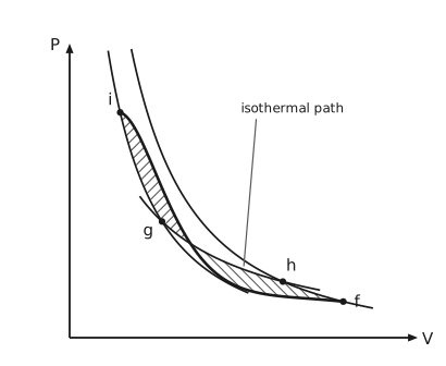
Figure 4 The reversible zigzag that replaces an arbitrary reversible path. Pressure is on the vertical axis and volume on the horizontal axis. Four states are marked with dots. A heavy curve falls from \(i\) at the upper left to \(f\) at the lower right: this is the arbitrary reversible path, and it wanders, rising above the zigzag over the first third of its length and sagging below it over the rest. Two lighter curves are the adiabats. The left one passes through \(i\) and through \(g\) below it; the right one enters at the top of the frame and passes through \(h\) and then \(f\). A third lighter curve is the isotherm, a hyperbola, labelled “isothermal path” by a leader line; it runs from \(g\) across to \(h\), so the zigzag \(i \to g \to h \to f\) descends the left adiabat, crosses along the isotherm, and descends the right adiabat. Two areas lie between the path and the zigzag and are hatched in opposite directions: the first, left of the point where the two cross, is the area by which the path runs above the zigzag, and the second, right of that point, is the area by which it runs below. The isotherm is placed so that the two are equal.
Entropy
For an arbitrary reversible, cyclic process, for example ABCDA (Figure 5), we want to evaluate the contour integral \(\oint \frac{δQ}{T}\) around the closed cycle. To do that, we divide the cyclic process into many small segments by drawing adiabats that intercept and demarcate the terminal points of the segments. For example, the adiabat \(mn\) marks \(s\) and \(u\) on the closed curve. We then draw isothermal paths according to the theorem of Clausius that intercept the adiabats and have the same heat interactions as the path segment on the original cyclic process. For example, \(op\) is such an isothermal path, representing the interactions with some heat reservoir at \(T_{B}\); \(op\), as well as rops, has the same heat interactions as \(rs\). Now consider the mini Carnot cycle rops-unwv: it has the same heat interactions as the original system during \(rs\) and \(uv\). Therefore
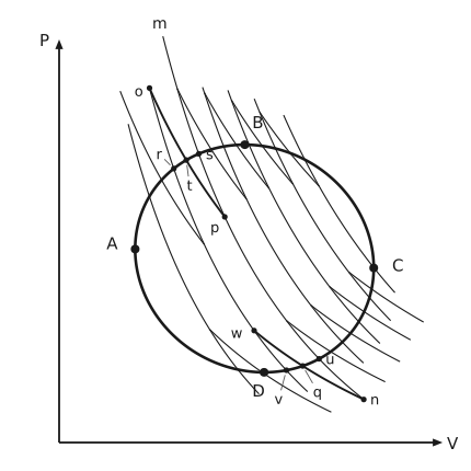
Figure 5 A reversible cycle divided into mini Carnot cycles by a family of adiabats. Pressure is on the vertical axis and volume on the horizontal axis. A heavy closed curve carries the four marked states of the cycle: A at its leftmost point, \(B\) at the top, \(C\) at its rightmost point, and \(D\) at the bottom. A family of seven adiabats, each a falling curve of \(PV^{γ}\) constant, cuts across the closed curve and extends a little beyond it at both ends. Between each neighbouring pair of adiabats runs an isotherm, a hyperbola of \(PV\) constant, drawn through the middle of the arc it replaces so that it cuts the closed curve there, and the small region each one closes off against the two adiabats is one of the mini Carnot cycles. One pair of adiabats carries the lettering. The right-hand one of that pair is labelled \(m\) at its upper end and \(n\) at its lower end, and it cuts the closed curve at \(s\) on the upper arc and \(u\) on the lower arc; the adiabat to its left cuts the curve at \(r\) above and \(v\) below. The isotherm from \(o\), on the left-hand adiabat above the curve, to \(p\), on the \(mn\) adiabat inside it, crosses the arc from \(r\) to \(s\) at \(t\). Below, the isotherm from \(w\), on the left-hand adiabat inside the curve, to \(n\), on the \(mn\) adiabat below it, crosses the arc from \(u\) to \(v\) at \(q\).
This implies a state function
Example 4.3
Problem
Prove that for an adiabatic process between defined states I and II of a closed system, the entropy change of the system must be equal to or greater than zero.
Proof. Consider a reversible process II → I, during which the heat interactions occur as part of an isothermal step, following the theorem of Clausius. The construction is shown in Figure 6.
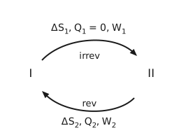
Figure 6 The adiabatic path from I to II and the reversible return. State I is at the left and state II at the right. A curved arrow along the top runs from I to II and is labelled “irrev”, with its three quantities written above it on one line: \(ΔS_{1}\), \(Q_{1} = 0\) and \(W_{1}\). A curved arrow along the bottom runs from II back to I and is labelled “rev”, with its quantities likewise written below it: \(ΔS_{2}\), \(Q_{2}\) and \(W_{2}\).
We can prove \(Q_2 \le 0\) by contradiction:
would violate the Kelvin-Planck statement of the second law (i.e., a perpetual-motion machine of the second kind, Figure 7).
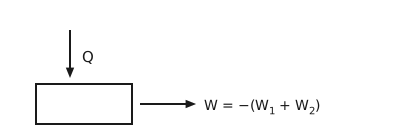
Figure 7 The device forbidden by the Kelvin-Planck statement. An arrow labelled \(Q\) carries heat down into a plain rectangular box, and a single arrow leaves the box to the right carrying work \(W = - \left(W_{1} + W_{2}\right)\). The box exchanges heat with one reservoir only.
Therefore
Since
it follows that
The second law
\(\mathrm{d}S \ge 0\) for an isolated system
\(\mathrm{d}S = 0\) for a reversible process
\(\mathrm{d}S > 0\) for an irreversible process
Isolated systems maximize their entropy, as shown in Example 4.3 above. Note that the second law applies only to isolated systems. Practically, we can always apply the second law to the universe, since the universe is by definition an isolated system:
The inequality holds for all real processes, while the equality is a limiting case of idealized reversible processes.
Entropy as a postulate
Alternatively, similar to the first law, we could postulate the existence of a state function called entropy that determines whether state B is adiabatically accessible from state A, that is, replacing Postulate II.
Consider Joule’s experiments: mechanical work is converted to internal energy and the system temperature rises. We however never observe the opposite: paddles turning to raise the weight with \(T\) decreasing, even though the first law is valid for both processes.
Adiabatic accessibility
There is a missing law and a “natural” order to the states of the system, such that it is impossible for a system to proceed from some states to others within an adiabatic enclosure.
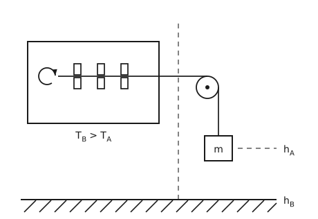
Figure 8 Joule’s experiment. A closed rectangular vessel on the left holds a paddle wheel: a horizontal shaft carrying three paddles, each a pair of blades set one above the shaft and one below it. At the inboard end of the shaft an open circular arrow gives the sense in which it turns. The shaft passes out through the right-hand wall of the vessel and wraps over a pulley just beyond it, and a cord leaves the pulley and hangs down to a block labelled \(m\). A dashed vertical line runs the height of the figure between the vessel and the pulley, clear of both. A dashed horizontal line runs from the block to the right, where it is labelled \(h_{A}\), marking the height of the weight in the initial state. A hatched horizontal line across the bottom of the figure is labelled \(h_{B}\), the height in the final state. The condition \(T_{B} > T_{A}\) is written below the vessel: the fluid is hotter after the weight has fallen.
Postulate
There is a state function \(S\left(U, x\right)\) that determines whether state \(B\) is adiabatically accessible from state A. \(S\) is a monotonically increasing function of \(U\):
In fact, this is the thermodynamic definition of temperature:
Expanding \(S\left(U, x\right)\) in its independent variables:
For a reversible process:
Substitution into \(\mathrm{d}S\) gives:
For an adiabatic reversible process, \(\mathrm{d}S = 0\) and \(δQ_{\text{rev}} = 0\). Therefore
We derived this equality using an adiabatic reversible process A → B, but since all quantities in the equation are state functions, this equality will hold for any reversible process connecting A → B. Therefore
Calculating entropy change, and the combined first and second laws
Since entropy is a state function, we shall find a convenient reversible process connecting the end states of interest.
\(T \mathrm{d}S\) equals \(δQ_{\text{rev}}\) but not \(δQ_{\text{irrev}}\).
Example 4.2
Problem
A bar of aluminum is placed in a large bath of ice and water (Figure 9). Current is passed through the bar until, at steady state, there is a power dissipation of 1000 W. A thermocouple on the surface of the aluminum reads 640 K. Film boiling is occurring at the interface with a subsequent, noisy collapse of the bubbles. What is the entropy change of the bar, water, and universe during 2 min of operation for this highly irreversible operation? Assume that there is ice remaining at the end of the 2 min.
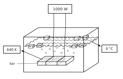
Figure 9 The aluminium bar in the bath of ice and water. An open rectangular tank is drawn in a shallow oblique view. The water surface is a band of waves across the tank, and blocks of ice float in it, each sitting with part of its body above the waterline and the rest below. Vapour bubbles rise through the water from the bar, which is the film boiling the problem describes. The bar is a slab lying near the bottom, drawn as a solid with its top face hatched and labelled “bar” by a leader line. Above the tank a box reads 1000 W, and two leads run down from it, through the water, and wrap right round the bar, the hidden part of each wrap drawn dashed. An arrow leaves the surface of the bar for a box reading 640 K, the thermocouple reading, and a second arrow leaves the water for a box reading 0 °C, the temperature of the bath.
For the bar:
There is no change in properties, so
For the water and ice, there is no \(p \mathrm{d} V\) or electric work:
so that
Imagine an alternative process that melts the same amount of ice reversibly by immersing the system in a heat batch maintained at 0 °C (Figure 10), causing the ice / water mixture to reach the same end state.
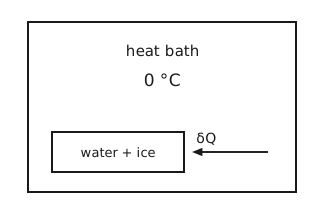
Figure 10 A reversible process that effects the same changes. A large box is labelled “heat bath” at 0 °C. Inside it, near the bottom, a smaller box is labelled “water + ice”. An arrow labelled \(δQ\) points from the bath into the smaller box, so heat passes reversibly from the bath to the water and ice.
Carnot cycle
Use the entropy balance to derive the efficiency of a reversible Carnot engine.
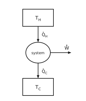
Figure 11 The Carnot engine. A box at the top is labelled \(T_{\mathrm{H}}\) and a box at the bottom is labelled \(T_{\mathrm{C}}\). Between them sits a circle labelled “system”. An arrow labelled \(\dot{Q}_{\mathrm{H}}\) carries heat down from the hot reservoir into the system, a horizontal arrow labelled \(\dot{W}\) leaves the system to the right, and an arrow labelled \(\dot{Q}_{\mathrm{C}}\) carries heat down from the system into the cold reservoir.
Second law for open systems: the entropy balance
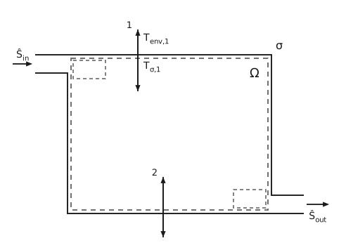
Figure 12 Open system for the entropy balance. A solid rectangle is the system boundary \(σ\), labelled at its upper right. A dashed rectangle a little inside it encloses the region Ω. A short duct enters at the upper left, flush with the top edge and open at both ends: the wall it shares with the boundary is not drawn, so it opens straight into the system, and its mouth is open to the surroundings. An arrow labelled \(\hat{S}_{\text{in}}\) carries entropy in with the incoming mass, and a dashed box of the same size as the duct, in the upper left corner of Ω, marks the element of mass \(\mathrm{d}m_{\text{in}}\). A second duct leaves at the lower right, flush with the bottom edge and open in the same way, with an arrow labelled \(\hat{S}_{\text{out}}\) carrying entropy out and a matching dashed box in the lower right corner of Ω marking \(\mathrm{d}m_{\text{out}}\). At station 1, on the top edge, a double-headed vertical arrow crosses the boundary: the boundary temperature there is \(T_{σ,1}\) and the temperature of the environment further out is \(T_{\text{env},1}\). At station 2, on the bottom edge, a second double-headed vertical arrow crosses the boundary in the same way.
State 1, at time \(t_{1}\):
State 2, at time \(t_{2}\):
Subtracting,
\(T_{σ,i}\) is the temperature at the boundary, which is often unknown. Instead, the temperature of the environment, \(T_{\text{env}}\), away from the boundary may be known.
Adding and subtracting the same sum over the environment temperatures:
which rearranges to
The last sum is always positive because the two cases go together:
If \(T_{\text{env},j} > T_{σ,j}\), then we must have \(δQ_{σ,j} > 0\);
If \(T_{\text{env},j} < T_{σ,j}\), then we must have \(δQ_{σ,j} < 0\).
Writing that sum as the entropy generated, which is therefore always greater than or equal to zero:
and in rate form,
For a reversible adiabatic system at steady state,
Example: minimum work to compress an ideal gas
Problem
Compute the minimum work required to compress an ideal gas adiabatically in a compressor, given \(P_{1}, T_{1}\), and \(P_{2}\).
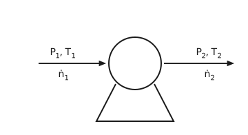
Figure 13 The compressor. A circle mounted on a wedge-shaped base is the compressor. An arrow entering from the left carries the feed at \(P_{1}, T_{1}\) and molar flow \(\dot{n}_{1}\). A horizontal arrow leaving to the right carries the discharge at \(P_{2}, T_{2}\) and molar flow \(\dot{n}_{2}\).
First law at steady state:
Entropy balance for a reversible compressor:
which follows from integrating \(\mathrm{d}\tilde{S} = \frac{\mathrm{d}\tilde{U}}{T} + \left(\frac{P}{T}\right) \mathrm{d}\tilde{V}\). Hence
where \(γ = \frac{C_{P}}{C_{V}}\).